In this lesson, you will learn how to find duplicates in Excel. It’s a quick way to find a large amount of data in just a second.

Applying conditional formatting to find duplicates

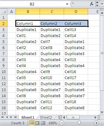
You have 3 columns of data and you want to highlight duplicates.

First select the whole table.

Go to the Ribbon. Home tab> Styles section. Click here to view Conditional Formatting > Highlight Cell Rules > Duplicate Values

A dialog box will appear. Choose how to highlight duplicates in Excel. I chose dark red text with a light red fill.

Excel highlights duplicates in your table.

Applying the match formula

Another way I know is to use the match function.

Excel includes a match function that allows you to find a value in a given range of cells. It is enough to dress the match function in logical functions and we will get such a formula

=NOT(ISNUMBER(MATCH(B3,$C$3:$C$8,0)))

As you can see in the picture above, Excel correctly identified the duplicates.

When the value is unique it displays TRUE. If it found a duplicate in column B, it returned FALSE.

Applying the countif formula

You can also use a formula to find duplicates in Excel. One commonly used formula is the COUNTIF function. Here are the steps for using the COUNTIF function:

1. Create a new column next to the column you want to check for duplicates.
2. In the first cell of the new column, enter the following formula: “=COUNTIF(A:A,A2)”. Replace “A:A” with the column that you want to check for duplicates, and replace “A2” with the first cell in the column.
3. Copy the formula down to the last cell in the column.
4. The formula will return a count of how many times each value in the column appears.
5. To highlight the duplicates, use conditional formatting as described above, but select the new column with the formula results instead of the original column.
6. The duplicates will be highlighted in the new column.

Using the “Remove Duplicates” Feature

1. Select the range of cells or columns that you want to check for duplicates.
2. Click on the “Data” tab in the ribbon menu.
3. In the “Data Tools” section, click on “Remove Duplicates”.
4. In the “Remove Duplicates” dialog box, select the columns that you want to check for duplicates and click on the “OK” button.
5. Excel will remove all duplicate rows and display a message indicating how many duplicates were removed.

It is important to note that the method you choose will depend on your specific needs and the size of your data set. For small data sets, using the “Remove Duplicates” feature or conditional formatting may be the quickest and easiest solution. For larger data sets, using a formula may be more efficient.

Additionally, if you have multiple columns that you want to check for duplicates, you will need to use a different method, such as using a formula or a VBA macro, to compare the values in multiple columns.

It is also important to consider the order of your data when checking for duplicates. If your data is not sorted, duplicates may not be detected accurately. To ensure accurate results, sort your data before checking for duplicates.

I am doing this Excel tutorial to help you solve such problems. I hope that I was successful and that my website will help you in many other matters.

Related posts:

How to Get Data from another Sheet? How to generate random text from the list? How to Use the Double Filter in Excel to Filter Data by Multiple Criteria