How to Highlight Duplicates in Excel: Ultimate Step-by-Step Guide
In data management, “duplicate” means two or more cells that contain the exact same value. However, Excel can be tricky – it counts different spaces, capitalization and formatting as unique, even if they look the same.
Highlighting duplicates in Excel is one of the most frequent and essential tasks in data analysis. It allows you to quickly audit your dataset, find matching records that need correction, or identify potential errors. The best way to do this is by using a combination of Conditional Formatting and custom formulas.
Method 1: Highlighting Duplicates with Conditional Formatting (The Quick Fix)
For the vast majority of users, Conditional Formatting is all you need. This method quickly applies a visual rule to highlight identical values.
Step-by-Step Instructions
- Select Your Data Range: Click and drag over all the cells (columns/rows) that contain data you want checked for duplicates.
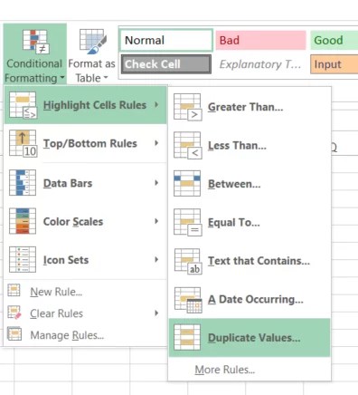
- Access Conditional Formatting: Go to the Home tab in the Excel ribbon. In the Styles group, click on Conditional Formatting.
- Select Duplicate Values Rule: From the dropdown menu, choose Highlight Cells Rules, then select Duplicate Values…
- Apply Formatting: A dialog box appears. You can leave Excel’s default (Red Fill) or click the formatting selector to change how you want the duplicates highlighted.
- Confirm: Click OK. All identical values in your selected range will instantly be marked.

Pro Tip: If you want to see the unique values instead, use the exact same process but select Unique in the Duplicate Values rule.
Method 2: Advanced Detection using Formulas (For Messy Data)
What if your data is spread across non-adjacent columns, or you need to count duplicates based on a combination of values? Conditional Formatting formulas are the power tool for this. This method is essential when simple highlighting isn’t enough.
Scenario: Highlighting Duplicates in Non-Adjacent Cells
If your duplicate check needs to compare Column A and Column D simultaneously, you must use a formula inside Conditional Formatting.
- Select the Target Range: Select only the column/cell range where you want the formatting to appear(e.g., select all of Column A).
- Access New Rule: Go to Home > Conditional Formatting > New Rule.
- Use a Formula: Choose the option “Use a formula to determine which cells to format.”
- Enter the COUNTIF Formula: Enter this specific formula (assuming your data starts in cell A2):
=COUNTIF($A:$A, A2)>1 - Set Formatting: Click the Format button and choose your desired highlight style. Click OK.
Why does this work? The formula COUNTIF counts how many times the value in cell A2 appears in the entire column ($A:$A). If that count is greater than 1, Excel applies your formatting rule.
Common XLB/Data Pitfalls and Solutions
Problem 1: Hidden Characters or Spaces
Excel sees “Name ” (with a space at the end) as completely different from “Name”. If your duplicate detection fails, check for these issues:
- Leading/Trailing Spaces: Use the TRIM() formula to instantly remove these invisible characters.
- Data Types: Are two columns storing numbers in different formats (one as text, one as actual number)? Convert them using VALUE() or ensure they are formatted consistently.
Problem 2: Case Sensitivity
The standard duplicate checker is NOT case-sensitive. If you have “APPLE” and “apple,” Excel treats them as duplicates. However, if your data must be strictly unique by casing (e.g., usernames), the basic CF rule won’t work.
Don’t Just Highlight – Remove Duplicates
Highlighting is great for finding errors, but if your goal is clean data, you need to eliminate the duplicates entirely. This is done using Excel’s built-in Data Cleanup tool.
- Select Data: Select the entire range of columns you want to de-duplicate (e.g., A through E).
- Access the Tool: Go to the Data Tab in the ribbon and click the Remove Duplicates button (it often has two arrows pointing back on itself).
- Select Key Columns: A dialog box will ask you which columns define a duplicate. Select all relevant columns. Excel will only consider rows duplicates if ALL selected fields match exactly.
- Execute: Click OK. Excel instantly deletes the redundant rows and leaves you with a perfectly clean, unique dataset.

Summary: When to Use Which Method
Understanding which method to use is key:
- Need a quick visual check? → Use Conditional Formatting (Method 1).
- Data is messy or non-adjacent? → Use the COUNTIF Formula Method (Method 2).
- Goal is clean data, not just visualization? → Use the Remove Duplicates Tool on the Data tab.