How to Create a Pivot Table from Multiple Sheets in Excel
Creating a Pivot Table from multiple sheets in Excel can be a powerful way to analyze data spread across different sources. You will learn how to make a Pivot Table from many sheets from this step-by-step guideline.
Creating pivot tables across multiple sheets
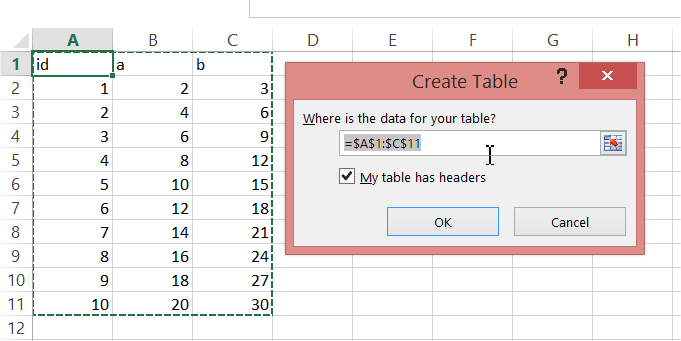
Start by navigating to each sheet containing your source data for the pivot table Create a Table from each set of data. Go to Insert -> Table.
Consider enabling the Data Model option. The Data Model allows you to work with larger datasets, create relationships between tables, and use DAX (Data Analysis Expressions) functions for more complex calculations.

Give each table a meaningful name in the “Table Name” box, like “SalesDataJan” or “SalesDataFeb”.

Create a Pivot Table. Go to Insert -> Pivot Table. Ensure the “Use this workbook’s Data Model” option is selected (this allows you to create relationships between tables from different sheets).

After creating the PivotTable, you’ll see the “PivotTable Fields” pane on the right.

You can create calculated fields directly within your Pivot Table. These calculated fields allow you to perform on-the-fly calculations based on existing fields in your Pivot Table.
Create a relationships between sheets
You need to create Relationships. This is a column which connects your tables. If you know data bases this is such a primary key in database.
Go to Ribbon. In the PivotTable Tools tab which appeared click Analyze -> Relationships.

Now let’s establish a new data model relationship between your multiple spreadsheet tables. For me it is id column which I have in my both tables. The most common are: order number, product number, id, name etc.

Your Pivot Table is ready. Feel free to create one for data from Multiple Sheets.


Leave a Reply