How to use Match function in Excel
The MATCH function allows you to determine the position of the search item in the range of cells. Excel is mainly used as a database to store large amounts of data, and frequently, you will have to search the Excel sheet for data.
As it is not at all practical to search the data manually, Excel offers a few functions to search the sheet for a specific value, like the MATCH function. The MATCH function returns the position of the searched value if successful, and returns the #N/A error value if the function is unsuccessful.
Table of Contents
Using the MATCH function in Excel

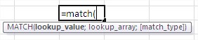
The Excel MATCH syntax is:
MATCH (lookup_value, range_lookup, [match_type])
- Lookup_value is an element we seek. This may be a number, text, logical value, or cell reference that contains one of these types of data.
- Range_lookup specifies the range of cells to be searched.
- Match_type is an optional argument (defaults to 1). It decides how to compare the values and looks for cells within the searched range. It may have the following values:
- 0 (exact match) – the result is given as the first value in the field of equal sought
- 1 (Less Than) – largest value ≤ lookup_value (requires ascending-sorted array)
- -1 (Greater Than) – smallest value ≥ lookup_value (requires descending-sorted array)
Match function examples
Let us use the function in the following example:

To find a person who is X years old, enter the following formula:
= MATCH (X, B2:B18, 0)
Looking for a person at age 50, we obtain a result of 9 – and thus the ninth person on the list is 50 years old. Typing an analogous formula for a person who is 60 years old, we get an #N/A error. This means that the value was not found.

To use a comparison of 1, sort the table columns by ascending age. To find the oldest person whose age does not exceed X years, enter the formula:
=MATCH (X, B2:B18, 1)
Since the table is a person aged 50 years, the function returns its position. In the case of finding a 60-year-old, get into the position of being 59 years old.

Let’s practice with these examples. Open Excel and save your file as match.xlsx. Enter details as in the following image.

Finding a string in a List: Click on cell F1 and enter the formula =MATCH(“MOU”,A2:A6,0).

The result here is 2, as “MOU” is in the second position within the range A2:A6.
Adjusting the Lookup Array: Click on cell F2 and enter the formula =MATCH(“MOU”,A1:A6,0).

The result is 3 because we shifted the starting point to A1, making “MOU” the third item in the array.
Wildcard matching in Excel MATCH: Click on cell F3 and enter the formula =MATCH(“Har*”,B2:B6, 0).

This returns 5, as “Harry” matches the pattern “Har*”.
Matching a Single Character: Click on cell F4 and enter the formula =MATCH(“Har?”,B2:B6, 0).

Here, the result is #N/A because there’s no such word in the list.
Matching a Single Character (Different Column): Click on cell F5 and enter the formula =MATCH(“LA?”,A2:A6, 0).

Now, the result is 4 because “LAX” matches the pattern “LA?”.
Sorted List and Type Parameter: Click on cell F6 and enter the formula =MATCH(48,D2:D6, 1).

The result is 2 because it returns the position of the largest value (45) less than or equal to 48.
Omitting the Type Parameter: Click on cell F7 and enter the formula =MATCH(62,D2:D6).

This returns 5 because it considers the default type parameter of 1.
Descending Order: Enter details in the A column as shown in the following image.

Click on cell F8 and enter the formula =MATCH(68,A9:A15,-1).

The result is 4, as it returns the position of the smallest value (75) greater than 68.
Descending Order (Different Value): Click on cell F9 and enter the formula =MATCH(43,A9:A15,-1).

Now, the result is 6, as 50 is the smallest value greater than 43.
Multiple instances in Excel MATCH: Click on cell F10 and enter the formula =MATCH(87,A9:A15,0).

The result is 2 because it returns the position of the first instance of 87.
Combine MATCH with INDEX for powerful lookups: =INDEX(return_range, MATCH(lookup_value, lookup_array, 0))

Leave a Reply