Understanding OLE Action in Excel
Do you want to connect your spreadsheet with another application? Would you like to know how Excel interacts with other programs? This is my experience about ole action in Excel for you.
The Largest Excel Knowledge Base ✅ The Best Place to Learn Excel Online ❤️
Do you want to connect your spreadsheet with another application? Would you like to know how Excel interacts with other programs? This is my experience about ole action in Excel for you.
Excel is always a great tool to play with numbers more than texts. Thus, a feature like, spell check is often overlooked compared to text editors. But it is one of most important features that Excel offers to its users to correct any error in texts instantly.
This ultimate guide covers up on how to use spell check in Excel by leveraging the options available for you in your workbook.
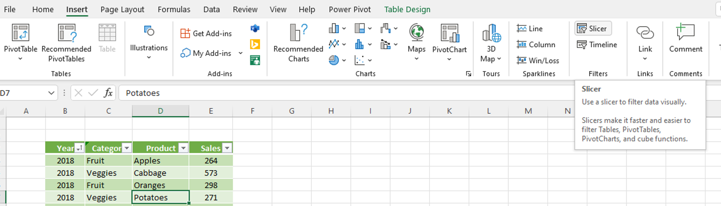
When it comes to data analysis, Excel is one of the most popular software programs available. And for good reason – it’s relatively easy to use and can be extremely helpful in a variety of different settings. However, if you really want to get the most out of your Excel usage, it’s important to learn about all of the features that the program has to offer. One of the most helpful features that you may not be aware of is called a slicer.
DAX expressions (Data Analysis Expressions) is the formal language for writing formulas in Power Bi, Power Pivot and in Excel data models. This language is made up of functions, constants, and operators.
You can use DAX to define custom calculations for Calculated Columns and for Measures (also known as calculated fields). It also allows you to calculate values, create relationships between tables, and more.
In this article, you will learn to create a grid in Excel:
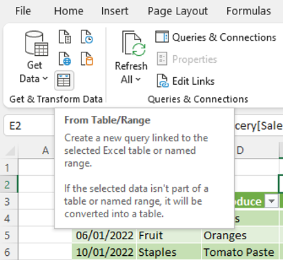
Power Query is a powerful data connectivity and data transformation tool that is available in Microsoft Excel. It allows you to connect to a wide range of data sources, such as spreadsheets, databases, and cloud services, and to easily manipulate, shape, and transform the data to meet your needs.
You learn to install and use Power Query in Excel.
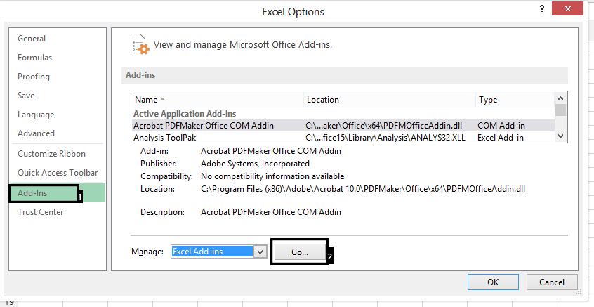
The Analysis ToolPak is an Excel add-in that provides advanced data analysis tools for Excel. To use the Analysis ToolPak in Excel, you need to first install and activate it. By following these steps, you will be able to use Analysis ToolPak add-in.
The Watch Window in Microsoft Excel is a feature that allows you to monitor the values of cells while you work in a different part of the workbook. The Watch Window is particularly useful when you are working with large, complex spreadsheets, and you need to keep an eye on the values of specific cells. With the Watch Window, you can track the values of cells without having to scroll back and forth between different parts of the worksheet.
Here is how to use Watch Window in Excel.
In Excel, you can define custom number formats to display numbers in a specific way. This can be useful for formatting currency, percentages, dates, and times.
You will learn how to define a custom number format in Excel. You will also learn about the most commonly used codes for custom number formats.