DAX expressions (Data Analysis Expressions) is the formal language for writing formulas in Power Bi, Power Pivot and in Excel data models. This language is made up of functions, constants, and operators.

You can use DAX to define custom calculations for Calculated Columns and for Measures (also known as calculated fields). It also allows you to calculate values, create relationships between tables, and more.

In this Excel tutorial lesson, we will discuss what DAX Expressions are and how you can use them in your Excel spreadsheets. We will also look at some of the benefits of using DAX Expressions and explore a few real-world applications.

Finally, we will provide you with some information on how to get started using DAX Expressions in your spreadsheets.

Why Use DAX Expressions?

There are many benefits to using DAX Expressions in your Excel spreadsheets. DAX Expressions offer several advantages over other methods of data analysis and modeling.

• DAX expressions are easy to learn and use.
• They allow you to perform complex calculations on your data with ease.
• They make it easy to create relationships between tables.
• They are very efficient, meaning that they can handle large data sets without slowing down your computer.
• They allow you to use formulas across more than one table and to make formulas by using existing formulas.

What Information Do You Need to Know to Get Started Using DAX Expressions in Your Spreadsheets?

If you want to start using DAX expressions in Excel, there are a few things you need to know first. First, you need to have a basic understanding of how DAX expressions work. Second, you need to have a data set that you can use to practice creating DAX expressions.

With these things in hand, you are ready to start using DAX expressions in your spreadsheets.

Preparing to Create DAX Expressions

Getting Data | Creating A Query

To create DAX expressions in Excel, we first need to load the data from your table(s) into the Data Model. For this article, we have sample data in the file – How To Use DAX (Data Analysis Expressions) Functions In Excel.xlsx.

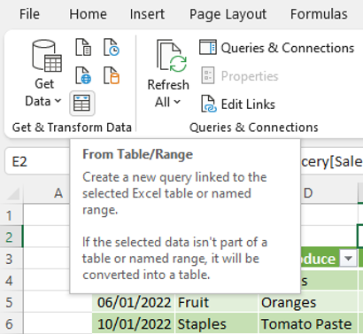
Open the sample data file. Click any cell in the Q1Data table, on the ribbon, click Data, Get & Transform Data group, click From Table/Range.

If you are seeing the Create Table dialog, this means your cursor was outside the table. Select your table including the headers, click My table has headers, click Ok.

The Power Query Editor opens with the Q1Data table displayed. You can use the query at this stage to edit the table as you wish – removing duplicate records/columns, adjusting format of text/numbers, etc. – so only the required data will be loaded into the Data model.

Loading Tables Into A Data Model

Once the query has been edited to your requirements, we can load the data into the data model. Using the Close & Load To option we can also create a Pivot Table at the same time.

On Home tab, click Close and Load To…

The Import Data dialog opens, select PivotTable Report, New worksheet and Add this data to the Data Model, click Ok.

The Power Query Editor closes, you are back in Excel on a new tab created for the PivotTable. The PivotTable Fields pane is active. On the right of the window the Queries & Connections pane is open. The Connections tab is visible.

Rename this worksheet tab Q1Data PT, to differentiate it from table tab.

Getting Data, Creating A Query, Loading Data For Subsequent Tables.

Repeat the steps for all the tables you wish to include in your data model. In this case, we need to repeat the steps above for the Region table too.

1. Click any cell in the Region table, on the ribbon, click Data, Get & Transform Data group, click From Table/Range. If you are seeing the Create Table dialog, this means your cursor was outside the table. Select your table including the headers, click My table has headers, click OK.
2. The Power Query Editor opens with the Region table displayed. Any other tables are included in this query are in the left pane. You can use the query at this stage to edit the table as you wish – removing duplicate records/columns, adjusting format of text/numbers, etc. – so only the required data will be loaded into the Data model.

Loading Tables Into A Data Model

1. On Home tab, click Close and Load To…
2. The Import Data dialog opens, select PivotTable Report, New worksheet and Add this data to the Data Model, click OK.

The Power Query Editor closes, you are back in Excel on a new tab created for the PivotTable; the PivotTable Fields pane is active. The Queries & Connections pane is on the right; the Connections tab is visible.

Rename this worksheet tab Region PT, to differentiate it from table tab.

Creating A PivotTable From A Data Model

On the the Q1Data PT tab, click in the PivotTable template area to view the PivotTable Fields Click the Product field checkmark, Excel places Product into the Rows area and on the PivotTable.

Creating A DAX Expression Through Measures

DAX Expressions Syntax

Before we create an expression, let’s review the syntax of DAX and the aspects that make up a formula.

The syntax for DAX expressions is =FUNCTION(TableName[Column name]). 

Measures

• Formulas created using DAX expressions are known as Measures. Measures can be entered/created in formula bars or in Measure dialog boxes which we will see later.
• Measure names must always be in square brackets [].
• Measure names can contain spaces.
• Measure name cannot be repeated within a model. Thus, it is not necessary to include the table name in a measure.

Functions

• Once you press equals (=), Excel presents you with a list of DAX functions that start with the letter you typed.
• Here’s a list of DAX functions https://docs.microsoft.com/en-us/dax/dax-function-reference

Table Name

• Enter all table names in brackets ()
• Unlike with Excel formulas you must enter the closing bracket when creating DAX expressions or you will receive an error.

Column Names

• Enter column names in square brackets [].
• When entering column names, a list of columns within the model appears for your selection.
• In Excel, we apply formulas to individual cells or ranges of cells. In DAX the formulas refer to columns of data or tables instead of cells.
• The names of your columns must be unique within your table; however, you can have multiple tables with identical column names, just include the table names to differentiate. For example, you can have two different columns name Sales, when using them in an expression use the table name to specify which of them you are referring to =Sum(Q1Table[Sales])+ (Q2Table[Sales]).

Creating A Measure

We are going to create a measure through the PivotTable, to count the units per order.

In the PivotTable Fields pane, right-click on the Q1Data table name, click Add Measure.

The Measure window opens, make the following entries:

• Table name – Q1Data, you could change the table here if required
• Measure Name – enter Units
• Value Description – enter Units per order

In the formula box we will enter the measure, once you type in the function a list of the tables and fields from the Data Model that is linked to this PivotTable appears.

You can adjust the zoom in this field if the text is too small, hold down CTRL and push the rollerball on your mouse forward.

Type =SUM(

Select the Table and column you want, in our case Q1Data[Sales]

The full expression is =SUM(Q1Data[Sales]) – unlike with regular Excel formulas, you must enter the closing bracket or you’ll get an error.

Enter the closing bracket.

In Category, click Number. Click Use 1000 separator, OK.

In the PivotTable Fields you’ll now see the Units measure under the list of columns.

Click the checkmark beside the Units measure; Excel adds it into the Value The PivotTable now includes the Units measure. The values here are total sales for each of the Product.

This measure allows us to view the subtotal of all the sales by product.

Let’s create a few more measures. Say a sales manager for this team wants to count the number of orders in the Q1Data table; we are counting each entry as an order in this example. They can create a measure to do that.

Right-click on the table name, click Add Measure. In the Measure window enter Number of Orders. Value description – counts each row as an order. Enter =countrows(

Type the letter ‘q’, click on the Q1Data name that appears, close the bracket. We don’t need to include and column name in this formula as its only counting the number of rows in the table.

The full expression is =COUNTROWS(Q1Data). Under Number click Use 1000 separator, click Ok.

The Number of orders measure now appears in the PivotTable Field list, click the checkbox to add the field to the PivotTable; Excel adds it into the Values area.

What we can see now is that for Laptops there were 4 orders with a combined total of 501 units.

Creating Formulas With DAX Expressions

Say a manager wants to know the average units per order, we can create a measure with a formula to give us that data.

Here’s where an advantage of DAX expressions comes in, we can use existing measures in a new measure/formula. In this case we’ll use the Number of orders measure to get the average units per order.

Right-click on the table name, click Add Measure

In the Measure window, Measure Name enter Ave units per order

In the Value Description field enter Units/Number of orders

In the measure pane enter =[

Excel lists the units measure as fx Units, select it.

Enter /[n and select the Number of orders measure.

Under Number click Use 1000 separator, select 2 in Decimal Places.

Tick the Ave units per order This column is added to the PivotTable.

Though we used division to create a new formula with existing measures, we can create formulas using other operators – addition, subtraction and so on.

Reusing A Formula/Measure

So currently we have the Average units per order by Product. We can use this measure to show the Average units per order by Salesperson.

Deselect Product, Units and Number of orders.

Select Salesperson. Now we have the average units per order by Salesperson by reusing the formula/measure created earlier.

Linking Data Tables | Creating Relationships Via Diagram View

The manager would like to know the average units per order by region, to compare the effectiveness the sales team in each region. The list of salespersons and the region they’re responsible for is in a separate table called Region.

The manager can use the Ave units per order measure for this comparison but first we need to create a link between the Q1Data and Region tables.

Click in the PivotTable. On the ribbon, Power Pivot tab, click Manage.

The Power Pivot for Excel window opens, there is a tab for Q1Data and Region.

On the Home tab, View group, click Diagram view.

Click on Salesperson in the Q1Data the label turns green, drag the cursor to the Salesperson field in the Region table.

The link is created, it starts out highlighted green, then changes to a one-to-many relationship, i.e., for each salesperson listed once in the Region table, they appear multiple times in the Q1Data table.

Close the Power Pivot for Excel window. In the Q1Data PT tab, click in the PivotTable. In the PivotTable Fields window click All, Excel displays the related tables.

Click the Q1Data listing with the little red query icon, deselect Salesperson. Open the Region list with the little red query icon, select region.

We now have the average units per order by region.

How to Edit/Delete Measures/DAX Expressions

Should you need to edit a measure there are a couple of ways to do this.

To edit a measure in the PivotTable Fields pane. Right-click on the measure, select Edit Measure, make your changes.

In the Power Pivot tab, click Measures, Manage Measures.

Select the measure to edit, click Edit, note you can also delete a measure in this view.

The measures window opens, edit as needed.

What Are the Real-World Applications of DAX Expressions?

DAX Expressions can be used for a variety of purposes. For example, you can use them to calculate values, create relationships between tables, and more. In the business world, DAX expressions are often used to create financial models. In the academic world, they may be used to analyze data sets in research studies.

DAX Expressions are a powerful tool that you can use in Excel to analyze and model data. In this blog post, we discussed what DAX Expressions are and how you can use them in your Excel spreadsheets. We also looked at some of the benefits of using DAX Expressions and explored some real-world applications. Finally, we provided you with some information on how to get started using DAX Expressions in your own spreadsheets! With this information, you are now ready to start using DAX expressions in your own Excel spreadsheets. Give it a try and see what you can create!

Do you have any tips for using DAX Expressions in Excel? And be sure to check out our other Excel tutorial posts for more tips and tricks on using Microsoft Excel. Thanks for reading!