How to use Anova in Excel
Anova means Analysis of Variance. In this Excel tutorial, you will teach yourself how to perform Anova.
ANOVA is used to test for the significance of the difference between the means of two or more samples.
In order to be able to perform the analysis of variance, 3 conditions must be met:
- independent samples;
- from a normal population;
- homogeneity of variance.
Table of Contents
Anova Single Factor test
Data preparation
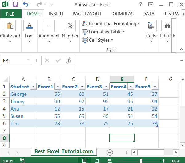
Let’s start from preparing data table.
- Organize your data into columns, with each column representing a group of data.
- Label each column with a descriptive heading.
- Make sure that each column contains an equal number of observations.
Here is an example:

Data analysis
Next go to the ribbon to the Data tab. Click Data Analysis button.

If you don’t have this button it means that you have to install Analysis ToolPak add-in.
Anova calculations
New dialog box appears. Click Anova: Single Factor option.

Select Input Range which is your data table (only numbers). In my sheet it is $B$2:$F$6
In the Alpha box, enter the level of significance you want to use for the test. A common value is 0.05.
Note: If your data has headers, check the Labels in First Row check box.

Anova test appears in the new worksheet.
The ANOVA analysis will generate several results, including the F-value, the degrees of freedom, and the p-value. The F-value measures the ratio of the between-group variability to the within-group variability, and the p-value is the probability that the difference between the means is due to chance. If the p-value is less than the level of significance, you can conclude that there is a significant difference between the means of the groups.

Anova test could be useful for statistics of some sets of data. Excel does it really well.
Anova two factor without replication test
Let’s learn how to perform Anova two factor without replication test.
Data preparation
Let’s start from preparing data table. Here is an example:

Data analysis
Next go to the ribbon to the Data tab. Click Data Analysis button.

New dialog box appears. Click Anova: Two-Factor Without Replication option.

Select Input Range which is your data table (only numbers). In my sheet it is $A$1:$F$5. My data table do have labels. As Alpha I left default 0.05.

Anova test appears in the Output Range I defined.

Anova two factor with replication in Excel
Let’s learn how to perform Anova two factor with replication test.
Data preparation
Let’s start from preparing data table. Here is an example:

Data analysis
Next go to the ribbon to the Data tab. Click Data Analysis button.

New dialog box appears. Click Anova: Two-Factor With Replication option.

Select Input Range which is your data table (only numbers). In my sheet it is $A$1:$F$5. In each example (group of students) I have 3 samples. As Alpha I left default 0.05.

Anova test appears in the Output Range I defined.

Anova two factor with replication test could be useful for statistics of some sets of data. Excel does it really well.


Leave a Reply