How to calculate p value in Excel
In this Excel tutorial, you will learn how to calculate p value in Excel.
What is a P-Value?
A p-value is a statistical measure that quantifies the probability of obtaining a result as extreme as, or even more extreme than, the one observed in your study if the null hypothesis were true. In essence, it tells you how likely it is that the observed results are due to random chance.
Step-by-Step Instructions
Have two sets of data ready, such as hours studied (independent variable, X) and exam scores (dependent variable, Y).
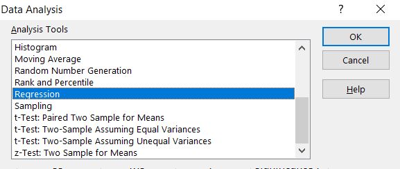
Click Data Analysis button and choose Regression.

Put input values. In my example, Y Range is for exam scores and X Range are hours studied.
As and Output Range choose where would you like to put results of Regression analysis in your sheet.

Here there are results of regression analysis.

P value of exam score is exactly 0.012304189. It suggests that there’s a statistically significant relationship between hours studied and exam scores at the conventional significance level.
You got also other values like Standard Error and Anova test.
Interpretation and Significance
Understanding the p-value is essential for data analysis and hypothesis testing. When you obtain a p-value from your regression analysis, you need to compare it against your chosen significance level, typically 0.05. If the p-value is less than 0.05, you can reject the null hypothesis and conclude that there is a statistically significant relationship between your variables. This means the observed relationship is unlikely due to random chance.
In our example with the p-value of 0.012, this indicates a strong statistical significance. The relationship between hours studied and exam scores is not merely coincidental but represents a genuine correlation. This type of analysis is invaluable for researchers, students, and professionals making data-driven decisions in various fields including education, business, and healthcare. Excel makes this complex statistical procedure accessible to everyone, regardless of their statistical expertise.


Leave a Reply