How to Perform ANOVA Two-Factor Without Replication in Excel: Statistical Analysis Guide
ANOVA, short for Analysis of Variance, is a powerful statistical technique for analyzing differences between groups. In this Excel tutorial, you’ll learn step-by-step how to perform an ANOVA two-factor without replication in Excel and master this essential Data Analysis Toolpak method.
Table of Contents
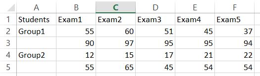
Data preparation
Organize your data in a table format, ensuring it includes the factors you want to analyze.

Data analysis
Navigate to the “Data” tab on the Excel ribbon.

Look for the “Data Analysis” button. Select “Anova: Two-Factor Without Replication” from the options.

Performing the Test
Once you’ve configured the settings, click “OK” to run the Two-Factor ANOVA without replication test.
When you run the Excel ANOVA two-factor without replication test, Excel will perform the analysis and present the results in your specified output range, providing critical insights into how different factors interact within your dataset.

Excel will perform the analysis and present the results in your specified output range. This test is valuable for statistically comparing sets of data, and Excel excels at executing it effectively.

By mastering this technique, you’ll be better equipped to analyze and interpret variances between different factors in your data.


Leave a Reply