Chart with combo box
In this Excel tutorial, you will learn how to insert chart with combo box.
Table of Contents
Adding a combo box for a chart
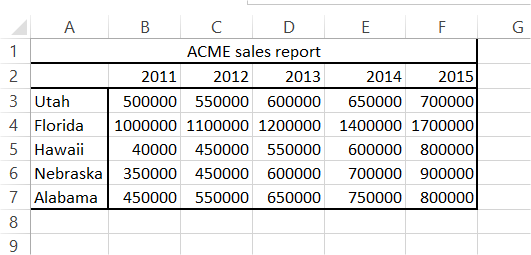
First, prepare a table with the data you want to show in the chart.

Copy and paste a list of arguments (countries in my example) to another column. You will use this table in the next steps.

Go to the ribbon to the Developer tab. Insert a combo box using VBA controls.

Right-click your combo box and select Format Control.

Now set the properties of your combo box. Input range are your values from the list you created at the beginning. Set also a Cell link wherever you want.

Cell link is here. There will be a velue you will need for your chart.

Combo box works since here. You can try it out. In the cell link there will be a value 1 – 4. It depends on country you will choose.
Copy first column of your table and paste it below.

In B column header (B16 in my example) write this formula: =INDEX(list_of_countries, cell_link). In my example it is =INDEX(P3:P6;B14)
In B17 write another formula down. It is =VLOOKUP(product_name, data_table, cell_link + 1, FALSE). Here it is =VLOOKUP(A17;$A$3:$E$12;$B$14+1;FALSE)
Next drag and drop this formula down. In this way, you create a new helper table that repeats the same data as your original table.

Creating a combo box chart
At this point, most of the work is done. Next, you will create the chart.
Highlight your table with sales data but only A and B column.

Go to the ribbon and create a column chart. This is how the chart looks.

Your combo box now works and changes the data in the chart. Go there and change a value from drop-down list. Your chart will change like mine here.

Finally, your interactive chart with a combo box is ready to use.


Leave a Reply