How To Calculate Variation Ratio Test (aka. F-Ratio test)
The Variation Ratio test, also known as the F-Ratio test, is a statistical method used to compare the variances of two samples drawn from different populations. This test helps you determine whether the variations (or spreads) of two samples are statistically equal. Understanding and applying this test is essential for statistical analysis work in Excel.
You need to activate the Analysis ToolPak in Excel to access the F-test function.
To run the F-test use sample data file Variation Ratio Test sample data.
Adding the Analysis ToolPak to the Data tab
Look at your Data tab in the ribbon. If you see an Analysis section with a Data Analysis button, the Analysis ToolPak is already active and you can skip the activation steps. If the Analysis section is not visible, follow the activation steps below.
1. In Excel, click File.
2. Click Options.
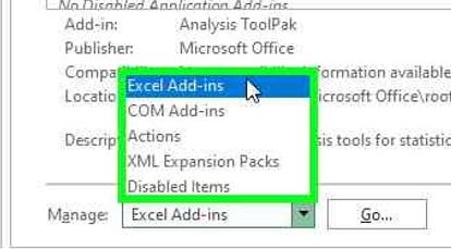
3. In the Excel Options window click Add-ins, in Manage select Excel Add-ins, click Go.

4. The Add-ins window opens, select Analysis ToolPak.

5. The Analysis section is now active on the Data tab.

Running the Variation Ratio / F-Test
1. Open the Variation Ratio Test sample data spreadsheet.
2. On the Data tab, click Data Analysis, then select F-test Two-Sample for Variances, click OK.

3. The F-test Two-Sample for Variances, window opens, click the Variable 1 Range arrow.

4. The window contracts to the Variable 1 Range field, select C4:C9, then click the arrow again.

5. Click the Variable 2 Range arrow, select D4-D9, click the arrow again.

6. Click Labels. In Output options click the Output Range arrow.
7. Select Cell F4, click the arrow again, click OK.
![]()
8. Excel displays the F-test results.

Quick reference guide
Steps to add the Analysis ToolPak
- In Excel, click File.
- Click Options.
- In the Excel Options window click Add-ins, in Manage select Excel Add-ins, click Go.
- The Add-ins window opens, select Analysis ToolPak and click OK.
- The Analysis section is now active on the Data tab.


Leave a Reply