How to Refresh Data in Pivot Table
In this Excel tutorial, you learn how to refresh pivot table with new data. You need this to analyze the data after the update.

Excel Skills Simplified: Tutorials That Actually Work
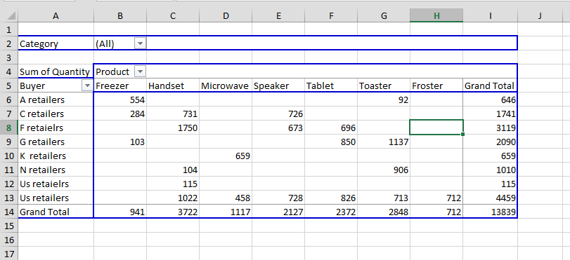
In this Excel tutorial, you learn how to refresh pivot table with new data. You need this to analyze the data after the update.
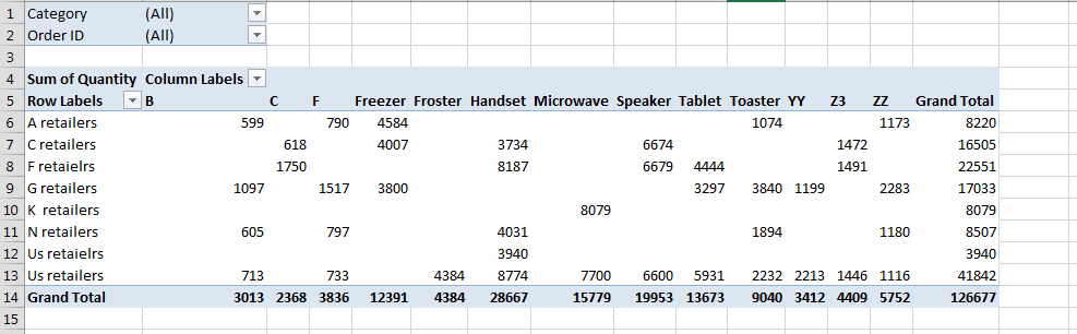
Pivot tables are a powerful tool in Excel that can be used to summarize and analyze data. One of the features of pivot tables is the ability to filter the data. This can be useful for finding the top 10 values in a particular field.
We will show you how to filter the top 10 values in a pivot table in Excel.
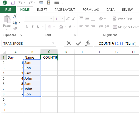
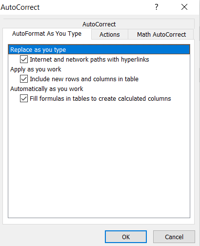
Excel has autocorrect data input turned on by default. After pasting the number into the cell, it is automatically replaced with the date. If the Excel number has a similar length as the date, it will go crazy and change the number to a date.
This changes the contents of the cell. A strange date appears instead of a number. These are often dates from hundreds of years ago or from the future.
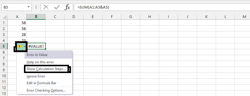
To show calculation steps in Excel, you can use the “Evaluate Formula” feature. Here’s how to use it:
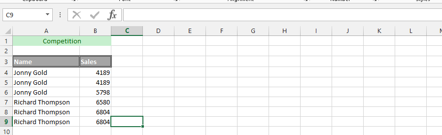
Showing the yes/no value in the Pivot Table has multiple steps to it. See how to do that in Excel.
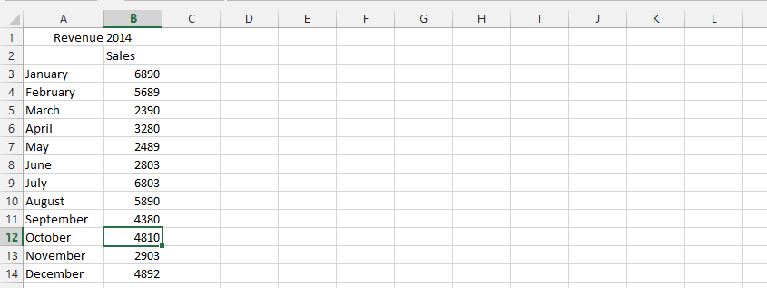
Win-loss data analysis in Excel can be done using the Quick Analysis tool, which is a feature that allows you to quickly analyze and visualize data in your worksheet. Here’s how to perform win-loss data analysis using Quick Analysis:
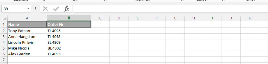
Learn how to increment row number in Excel formulas using ROW() and OFFSET() functions. This comprehensive tutorial teaches you how to create dynamic formulas that automatically adjust and increment row ranges. Master the techniques to increment row numbers for more flexible and powerful Excel calculations.
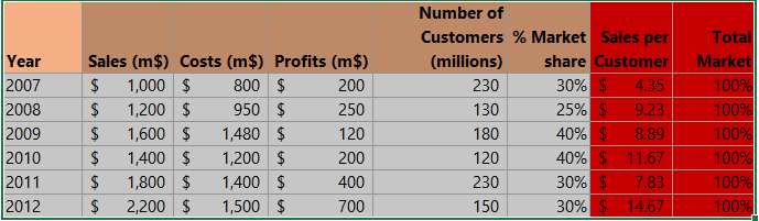
To create a dynamic Pivot Table that refreshes automatically, you need to start with data in a table format. The table must have headers, and the data must be in a consistent format.