Pivot tables are a powerful tool in Excel that can be used to summarize and analyze data. One of the features of pivot tables is the ability to filter the data. This can be useful for finding the top 10 values in a particular field.

In this article, we will show you how to filter the top 10 values in a pivot table in Excel.

Step 1: Open the pivot table

The first step is to open the pivot table that you want to filter.

Step 2: Select the field that you want to filter

The next step is to select the field that you want to filter. This is the field that you want to find the top 10 values for.

Step 3: Click on the value filter button

Once you have selected the field, you need to click on the value filter button. This button is located in the PivotTable Analyze group on the PivotTable Tools tab.

In the value filter menu, select the Top 10 option.

You can then set the criteria for the top 10 filter. This includes the number of items to display and the sort order.

Step 4: Click OK

Once you have set the criteria, click OK. The pivot table will be filtered to show the top 10 values for the selected field.

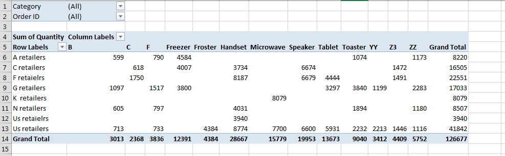
Here are some additional tips for filtering top 10 values in a pivot table:

• You can also use the Advanced Filter option to filter top 10 values in a pivot table. This option gives you more control over the filtering criteria.
• You can filter top 10 values in multiple fields by repeating steps 2-6 for each field.
• You can also filter top 10 values based on other criteria, such as date or time.

By following these steps, you can easily filter the top 10 values in a pivot table in Excel. This can be a useful way to find the most important data in your pivot table.

How to Filter Pivot Table Data by Multiple Criteria

In addition to filtering by the top 10 values, you can also filter pivot table data by multiple criteria. This can be useful for finding specific data points or for creating more detailed reports.

To filter pivot table data by multiple criteria, you can use the Advanced Filter option. The Advanced Filter option allows you to specify the criteria for the filter in a dialog box.

To use the Advanced Filter option, follow these steps:

1. Select the pivot table that you want to filter.
2. Click on the Data tab.
3. In the Sort & Filter group, click on the Advanced Filter button.
4. In the Advanced Filter dialog box, select the Range that you want to filter. This is the range of cells that contains the pivot table data.
5. In the Criteria Range, enter the criteria for the filter. The criteria can be a single value, a range of values, or a more complex expression.
6. Select the Filter option that you want to use. You can filter by the top 10 values, the bottom 10 values, or by custom criteria.
7. Click OK. The pivot table will be filtered to show the data that matches the criteria.

Here are some additional tips for filtering pivot table data by multiple criteria:

• You can use the AND and OR operators to combine criteria. For example, you could filter for products that are in the “Top 10” and that have a price of less than $100.
• You can use the Wildcard characters to match multiple values. For example, you could filter for products that start with the letter “A”.
• You can use the Date and time functions to filter for data based on a specific date or time range.

By following these steps, you can easily filter pivot table data by multiple criteria. This can be a useful way to find specific data points or for creating more detailed reports.

Related posts:

Counting unique values in pivot table How to Do to the Power of in Excel How to Run Cohort Analysis in Excel