How to HLOOKUP Multiple Rows?
If you’re familiar with VLOOKUP, HLOOKUP should come fairly easily. Rather than looking up values across columns, HLOOKUP allows you to look up values across rows. Pull in specific data quickly using an HLOOKUP formula, and capture data quickly across many rows.
Rather than manually looking up data, HLOOKUP reviews data in a specific range of rows and pulls in a specific data element that you identify. To help you get started with HLOOKUP, let’s take a look at how you can use it to look up data across multiple rows.
The HLOOKUP function in Microsoft Excel is a horizontal lookup function that allows you to search for a specific value in the first row of a table and return a value in the same column from a specified row. By default, the HLOOKUP function returns a single value. However, you can use the HLOOKUP function in combination with other functions or formulas to return multiple values.
Why Use HLOOKUP?
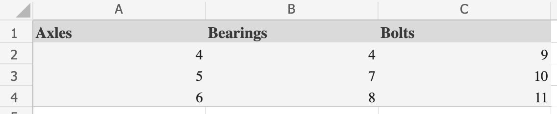
A HLOOKUP is a function that allows you to pull specific data from cells identified by the row they’re in. This is a useful function when you want to identify a value compared to something in one of the top rows of a table. The function pulls the specified data into a row below the comparison value. For example, let’s look at the simple dataset below. The cart identifies the number of axels, bearings, and bolts for manufacturing purposes.
Multiple Hlookup formula
We can use HLOOKUP to identify a specific cell in any of the rows beneath the headers. Let’s say we want to identify the number of bearings for the third line item. To do so, we would use the following formula:
=HLOOKUP(B1,A1:C4,4,FALSE)
In this example, we are identifying column B as the source column by entering B1. This means we are looking up Bearings. Next, we identify the entire range of the table. This captures the full data range for the function to search.
Finally, we need to identify the row number to return to. In this example, we are returning the fourth row, which is the header row plus the three data rows below it. When we enter the above formula, the output is 8, which is the third line item in the Bearings column.
Using an Array Formula
An array formula is a special type of formula that returns multiple values. To use the HLOOKUP function in an array formula, you need to wrap the HLOOKUP function in the INDEX and MATCH functions, and press Ctrl + Shift + Enter to create an array formula. Here’s an example:
=INDEX($B$2:$D$5, MATCH(A7, $B$1:$D$1, 0), {1,2,3})
This formula searches for the value in cell A7 in the first row of the table ($B$1:$D$1), and returns the corresponding values from rows 2 to 5 in the same column ($B$2:$D$5).
Leave a Reply