How to use Sparklines in Excel
In this Excel tutorial, you’ll learn how to use Sparklines in Excel – mini charts that show data trends within individual cells. Sparklines in Excel provide a fast way to visualize trends in data, making them ideal for dashboards, reports, and financial spreadsheets.
Creating Sparklines
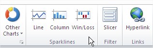
To insert a Sparkline in Excel, click inside your data range, then go to Insert > Sparklines and choose the Sparkline type (Line, Column, or Win/Loss).

The Create Sparklines dialog box will appear, prompting you to select your data and location range.

In the Data Range box, select the range of cells that contain the values you want to visualize with Sparklines.
In the Location Range textbox, identify where you want to insert the sparkline.
You can create multiple Sparklines in Excel by selecting rows individually or by using AutoFill to apply Sparklines across several rows.
Types of Sparklines
There are three primary types of Sparklines in Excel:
Line Sparklines
Line Sparklines are best for showing trends over time and work well with continuous datasets in Excel. Line Sparklines display a series of data points as a simple line, with the height of the line indicating the data value.

Column Sparklines
Column Sparklines resemble bar charts and are used to visualize categorical or comparative data within a row. They display a series of columns, with the height of each column representing the data value.

Win / Loss Sparklines
Designed for data sets with only two values (e.g., win/loss results or binary data), Win/Loss Sparklines display a series of small dots. Positive values are shown as dots above the line, while negative values appear below the line.

Highlighting Specific Points
You can customize Excel Sparklines by highlighting key points like high, low, first, last, or negative values. Use the Show group in the Sparkline Design tab to add markers for high, low, or other specific data points.
For instance, to highlight negative values in a Sparkline, select the “Negative Points” checkbox.

Customizing Sparklines
You can format Sparklines in Excel by changing their color, style, and size to match your spreadsheet layout. The “Sparkline Options” group on the “Design” tab provides options for changing marker color, line color, fill color, and border style.
You can also modify the Sparkline’s size by dragging the sizing handles.

Removing Sparklines
To delete Sparklines in Excel, do not press the Delete key – it won’t remove them. Instead, select the cells with the sparklines, right-click, and choose ‘Sparklines’ followed by ‘Clear Selected Sparklines’.

Alternatively, you can achieve the same result by selecting the sparklines, which will reveal the ‘Sparkline Tools Design’ tab on the ribbon. Within the ‘Group’ section of this ‘Design’ tab, you’ll find the ‘Clear’ option.

The Sparkline location range defines the exact cells where each Sparkline chart will appear in your worksheet. You can define the location range when creating Sparklines or modify it afterward.


Leave a Reply