How to Calculate Skewness in Excel
In this Excel tutorial lesson, you will learn what skewness is and how to calculate skewness in Excel application.
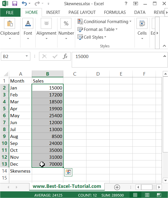
To find the skewness in Excel, please prepare some data tables.

Table of Contents
Calculate Skewness using the SKEW function
Excel provides a built-in SKEW function that allows you to calculate skewness in Excel with a simple formula. The syntax is:
=SKEW(number1, [number2], …)
To demonstrate how to use the SKEW function formula in Excel, here’s the formula: =SKEW(B2:B13)

A skewness value significantly greater than 0 (skewness > 0) indicates right-skewed (positively skewed) data. In this sales example, it suggests that sales were often significantly lower than the average. A positive skewness indicates that the distribution of sales data has a longer tail on the right side. This suggests that while there might be a few months with very high sales, the majority of months experienced sales below the average.
Calculate Skewness using Data Analysis ToolPak Add-In
First, you need to make sure your Data Analysis Toolpak Add-In is installed. Here is the lesson on how to install Data Analysis Toolpak Add-In.
Go to Ribbon to the Data tab. Click the Data Analysis button.

A new window appears. Choose Descriptive Statistics and click OK.

Enter the proper parameters:
- Input Range – range of your data ($B$1:$B$13 in my example).
- Labels in first row – there are labels in my data table.
- Output Range – choose where you want to get your skewness calculated (I chose the same Sheet $E$1:$F$15).
- Summary statistics – make sure it is checked.

And this is how you see my statistics summary. Skewness is calculated in row 10. The result is the same as in Example 1 where we checked how to calculate Skewness using the SKEW Excel function.

While the formula 3 * (Mean – Median) / Standard Deviation (Pearson’s coefficient) approximates skewness, Excel’s SKEW function provides a more accurate calculation. The SKEW function and the Data Analysis ToolPak use a different formula involving the third moment, which is the standard method for calculating sample skewness. Therefore, while the Pearson coefficient can give a rough idea, the SKEW function is the preferred and more precise way to calculate sample skewness in Excel.


Leave a Reply