We can use Mean Squared Error (MSE) to compare forecasted values to actual values, for example, comparing actual sales to forecasted figures. The lower the MSE score, the closer the forecast is to the actual results, and so MSE checks the accuracy of the forecast.

What is MSE?

In MSE the difference between the actual and forecasted value is squared; the total of all the squared values within the period is then divided by the number of values.  We square the results to prevent negative results.

We can use the SUMXMY2 function to sum the squares of the differences between the actuals and forecasts and then divide this sum by the number of values in the period.

To run this function, you will need a spreadsheet with actual values and forecast values.

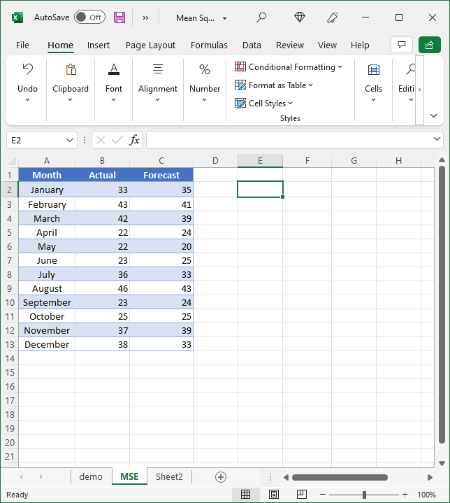
For the purposes of this guiden sample data has been created for you to use. In the sample data, the scenario is of a manager of a car dealership wishing to gauge the accuracy of the sales forecast.

Steps to calculate the MSE

The steps below will take you through the process using some sample data. A quick reference guide is available at the end of this document.

1. Open the Mean Squared Error – sample data Excel spreadsheet.

2. Click where you’d like the results to appear. Use E2 for this example.

3. In E2 type =SUMXMY2(

4. Select the first array, the values in the Actual column, cells B2:B13 – type a comma ‘,‘.

5. Select the second array, the values in the Forecast column, cells C2:C13. Close the bracket, but leave the cursor in E2.

6. Type ‘/Count(’ select B2:B13, close the bracket, press Enter.

7. Excel displays the result 417. This is the Mean Squared Error for the actual versus forecast car sales figures. This result shows that the forecast values were quite accurate, that is there was little error/difference between the actual value and the forecast.

Quick reference guide

1. Open the Excel spreadsheet containing the actual and forecast values you wish to analyse.
2. Click where you’d like the results to appear
3. Type =SUMXMY2(
4. Select the values in the Actual column, type a comma ‘,’
5. Select the values in the Forecast column, close the bracket, but leave the cursor in the cell.
6. Type ‘/Count(’ select the values in the Actual column, close the bracket, press Enter.
7. Excel displays the result; this is the Mean Squared Error for the actual versus forecast figures.

Calculate the mean squared error using LINEST function

Another method to calculate the Mean Squared Error in Excel is to use the “LINEST” function. The “LINEST” function is a built-in regression analysis tool in Excel that can be used to calculate the MSE.

Here is an example of how to use the “LINEST” function to calculate the MSE:

1. Assume the actual values are in column A and the predicted values are in column B.
2. In a blank cell, enter the “LINEST” function as follows: =LINEST(B2:Bn, A2:An, TRUE, TRUE). The first argument (B2:Bn) refers to the predicted values, the second argument (A2:An) refers to the actual values, the third argument (TRUE) specifies that the regression model should include the constant term, and the fourth argument (TRUE) specifies that the function should return additional regression statistics.
3. The “LINEST” function will return an array of values, where the MSE can be found in the bottom right corner of the array.
4. To extract the MSE, you can use the INDEX and MATCH functions, as follows: =INDEX(LINEST(B2:Bn, A2:An, TRUE, TRUE), 1, 2). The INDEX function returns the value in the first row and second column of the array returned by the “LINEST” function, which is the MSE.
5. The final result in the cell is the Mean Squared Error.

Calculate the mean squared error using POWER and AVERAGE functions

A third method to calculate the Mean Squared Error in Excel is to use the “POWER” and “AVERAGE” functions. These functions can be used to calculate the MSE as follows:

1. Assume the actual values are in column A and the predicted values are in column B.
2. In column C, subtract the predicted value from the actual value for each data point and square the result using the formula =POWER(A2-B2, 2).
3. In cell D2, average the squared differences using the formula =AVERAGE(C2:Cn), where “n” is the last row of the data.
4. The final result in cell D2 is the Mean Squared Error.

Note that this method gives you the average of the squared differences, rather than the sum of the squared differences as in the previous method. The result will be the same, as long as the number of observations is the same in both methods.

Calculate the mean squared error using SUMPRODUCT and COUNT functions

A fourth method to calculate the Mean Squared Error in Excel is to use the “SUMPRODUCT” and “COUNT” functions. These functions can be used to calculate the MSE as follows:

1. Assume the actual values are in column A and the predicted values are in column B.
2. In a blank cell, use the “SUMPRODUCT” function to calculate the sum of the squared differences as follows: =SUMPRODUCT((A2:A-B2:B)^2). The “SUMPRODUCT” function calculates the dot product of two arrays, which is equivalent to summing the element-wise products of the arrays. In this case, the two arrays are the differences between the actual and predicted values and their squares.
3. In a separate cell, use the “COUNT” function to count the number of observations as follows: =COUNT(A2:A).
4. In a third cell, divide the sum of the squared differences by the number of observations as follows: =SUMPRODUCT((A2:A-B2:B)^2)/COUNT(A2:A).
5. The final result in the cell is the Mean Squared Error.

Calculate the mean squared error using DEVSQ and AVERAGE functions

A fifth method to calculate the Mean Squared Error in Excel is to use the “DEVSQ” and “AVERAGE” functions. The “DEVSQ” function calculates the sum of squares of deviations from a mean value, and the “AVERAGE” function calculates the average value of a set of numbers. These functions can be used to calculate the MSE as follows:

1. Assume the actual values are in column A and the predicted values are in column B.
2. In a blank cell, use the “DEVSQ” function to calculate the sum of the squared differences as follows: =DEVSQ(A2:A-B2:B). The “DEVSQ” function calculates the sum of squares of deviations from the mean value, which in this case is the difference between the actual and predicted values.
3. In a separate cell, use the “AVERAGE” function to count the number of observations as follows: =AVERAGE(A2:A).
4. In a third cell, divide the sum of the squared differences by the number of observations as follows: =DEVSQ(A2:A-B2:B)/AVERAGE(A2:A).
5. The final result in the cell is the Mean Squared Error.

Calculate the mean squared error using SUM and SQRT functions

A sixth method to calculate the Mean Squared Error in Excel is to use the “SUM” and “SQRT” functions. The “SUM” function calculates the sum of a set of numbers, and the “SQRT” function calculates the square root of a number. These functions can be used to calculate the MSE as follows:

1. Assume the actual values are in column A and the predicted values are in column B.
2. In column C, subtract the predicted value from the actual value for each data point using the formula =A2-B2.
3. In a blank cell, use the “SUM” function to calculate the sum of the squared differences as follows: =SUM(C2:Cn^2), where “n” is the last row of the data.
4. In a separate cell, use the “COUNT” function to count the number of observations as follows: =COUNT(A2:A).
5. In a third cell, divide the sum of the squared differences by the number of observations and take the square root as follows: =SQRT(SUM(C2:Cn^2)/COUNT(A2:A)).
6. The final result in the cell is the Mean Squared Error. Note that this method calculates the Root Mean Squared Error (RMSE), which is the square root of the MSE.

Calculate the mean squared error using MMULT and TRANSPOSE functions

A seventh method to calculate the Mean Squared Error in Excel is to use the “MMULT” and “TRANSPOSE” functions. The “MMULT” function calculates the matrix product of two arrays, and the “TRANSPOSE” function transposes an array or range from rows to columns or vice versa. These functions can be used to calculate the MSE as follows:

1. Assume the actual values are in column A and the predicted values are in column B.
2. In a blank cell, use the “MMULT” function to calculate the sum of the squared differences as follows: =MMULT((A2:A-B2:B), TRANSPOSE(A2:A-B2:B)). The “MMULT” function calculates the matrix product of two arrays, which in this case is the difference between the actual and predicted values and its transpose. The result is a single value that is equal to the sum of the squared differences.
3. In a separate cell, use the “COUNT” function to count the number of observations as follows: =COUNT(A2:A).
4. In a third cell, divide the sum of the squared differences by the number of observations as follows: =MMULT((A2:A-B2:B), TRANSPOSE(A2:A-B2:B))/COUNT(A2:A).
5. The final result in the cell is the Mean Squared Error.

Calculate the mean squared error using pivot table

An eighth method to calculate the Mean Squared Error in Excel is to use a pivot table. A pivot table is a tool in Excel that allows you to summarize, sort, and analyze data in a flexible and dynamic way. The following steps describe how to use a pivot table to calculate the MSE:

1. Assume the actual values are in column A and the predicted values are in column B.
2. Select both columns of data.
3. Go to the “Insert” tab and click on “Pivot Table.”
4. In the “Create Pivot Table” dialog box, select “New Worksheet” as the location for the pivot table.
5. In the “Pivot Table Fields” area, drag the actual values column to the “Values” section and the predicted values column to the “Values” section as well.
6. Right-click on one of the values in the “Values” section and select “Value Field Settings.”
7. In the “Value Field Settings” dialog box, select “Difference From” and “Mean.”
8. In the “Base Field” dropdown, select the actual values column.
9. In the “Base Item” dropdown, select “Mean.”
10. Click “OK” to apply the settings.
11. The pivot table will display the mean of the differences between the actual and predicted values, which is equal to the MSE.

Note: The pivot table method provides a quick and easy way to calculate the MSE, but it may not be as flexible as using a formula-based method, as the pivot table displays the mean of the differences rather than the sum of the squared differences.

Calculate the mean squared error using SUMIF function

A ninth method to calculate the Mean Squared Error in Excel is to use the “SUMIF” function. The “SUMIF” function adds up the values in a specified range that meet a certain criteria. The following steps describe how to use the “SUMIF” function to calculate the MSE:

1. Assume the actual values are in column A and the predicted values are in column B.
2. In column C, subtract the predicted value from the actual value for each data point using the formula =A2-B2.
3. In a blank cell, use the “SUMIF” function to calculate the sum of the squared differences as follows: =SUMIF(C2:Cn, “>0”, C2:Cn^2), where “n” is the last row of the data. The “SUMIF” function adds up the values in column C that are greater than 0, which are the positive squared differences.
4. In a separate cell, use the “COUNT” function to count the number of observations as follows: =COUNT(A2:A).
5. In a third cell, divide the sum of the squared differences by the number of observations as follows: =SUMIF(C2:Cn, “>0”, C2:Cn^2)/COUNT(A2:A).
6. The final result in the cell is the Mean Squared Error.

Calculate the mean squared error using INDEX MATCH

A tenth method to calculate the Mean Squared Error in Excel is to use the “INDEX” and “MATCH” functions. The “INDEX” function returns the value of a cell in a specified range based on the row and column number, and the “MATCH” function returns the position of a value in a specified range. These functions can be used to calculate the MSE as follows:

1. Assume the actual values are in column A and the predicted values are in column B.
2. In column C, subtract the predicted value from the actual value for each data point using the formula =A2-B2.
3. In column D, square the differences in column C using the formula =C2^2.
4. In a blank cell, use the “SUM” function to calculate the sum of the squared differences as follows: =SUM(D2:Dn), where “n” is the last row of the data.
5. In a separate cell, use the “MATCH” function to find the position of the last value in the actual values column as follows: =MATCH(A2, A2:A, 0).
6. In a third cell, use the “INDEX” function to retrieve the number of observations based on the position found in step 5 as follows: =INDEX(A2:A, MATCH(A2, A2:A, 0)).
7. In a fourth cell, divide the sum of the squared differences by the number of observations as follows: =SUM(D2:Dn)/INDEX(A2:A, MATCH(A2, A2:A, 0)).
8. The final result in the cell is the Mean Squared Error.

In conclusion, there are many ways to calculate the Mean Squared Error (MSE) in Excel. Some of the methods include using formulas such as SUMPRODUCT, SUM, AVERAGE, and STDEV.P, as well as functions such as SUMIF, INDEX, and MATCH. Pivot tables can also be used to calculate the MSE by summarizing the difference between actual and predicted values. Each method has its own strengths and weaknesses, and the choice of method will depend on the specific requirements and data set being analyzed. Regardless of the method used, the MSE is a valuable metric for evaluating the accuracy of predictions and can provide important insights into the performance of predictive models.

Related posts:

Bisection Method Calculator in Excel How to Calculate Skewness in Excel How to calculate p value in Excel