How to Calculate Slope in Excel
In this article, we will learn how to calculate slope in Excel using the SLOPE function and manual slope calculation between two coordinate points.
Finding slope using Excel function
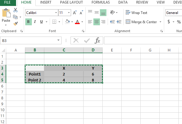
Let us demonstrate how to calculate slope from two points by using simple formulas and the SLOPE function in Excel. First, we’ll establish the coordinates of the two data points we’ll use to calculate our slope.

Calculate difference between x coordinates: C5-C4

The result is 2 in this example.

Now let us calculate difference between y coordinates: D5-D4

The result is 2 again.

Slope will be difference of Y coordinates divided by difference of X coordinates:

The Slope here is 1.

This was very simple approach, now we will do the same by using the slope function inbuilt in Excel:
SLOPE(known_y’s, known_x’s)
The SLOPE function syntax has the following arguments:
- Known y’s Required. An array or cell range of numeric dependent data points.
- Known x’s Required. The set of independent data points.

See in this example as we are typing the formula it is being guided by Excel with the comments below. The slope formula written as SLOPE(KNOWN Y’S,KNOWN X’S)
So the formula will be:
=SLOPE(D4:D5,C4:C5)
The final contents in the sheet with results is like:

Please find attached the Excel file for reference.
Finding slope from the chart
There is no need to use slope formula to find the slope. Sometimes it might be possible to find it from the graph.
Lets assume we have such data.

There is a measurement of some value. And you need to find the slope for the value. How to do that?
First, plot the line chart for that. Go to Insert > Line Chart.

You can see the simple chart.

Right-click the line and choose Add Trendline.

Menu pops in the right side of your screen. Choose “Display Equation on the Chart”.

And here is your slope.

Can’t you see that? If you forgot I will remind.
The equation of the trendline comes from the y = f(x) = ax + b
In this example y = 2.4706x – 10.941
a = 2.4706 and b = -10.941
a = slope = 2.4706
Note: b is the point where the line cross the horizontal line for x=0 point.


Leave a Reply