Monte Carlo simulation in Excel
In this Excel tutorial you will learn how to perform Monte Carlo simulation in Excel. It allows you to understand the impact of risk and uncertainty in financial models, project management, and forecasting.
Monte Carlo calculations
Let’s move on with calculations.
To calculate revenue I used =(400+RAND()*100)*215 formula:
- remember that number of clients is 400-500
- 400+RAND()*100 will generate random number between 400 – 500
- unit price is 215 and I need to multiply random number of clients in range between 400 and 500 to get total sales
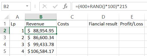
Apply formula to the entire column.
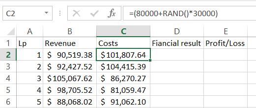
Next, calculate the costs. Simuilarly formula is =(80000+RAND()*30000) to generate random number in range 80,000 – 110,000.
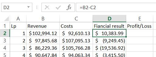
To calculate financial results you just need to know how to subtract in Excel. The formula is =B2-C2.
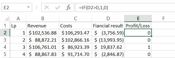
For the next Profit/Loss column we need to know if it is true or not. Let’s agree that for profit we will see 1 and 0 will be for loss. IF Excel function will do the job!
The formula is =IF(D2>0,1,0)
Now, we are able to calculate average of expected profit. Of course there is dedecated function for that. Average Excel function will calculate it.
The formula is =AVERAGE($D$2:$D$10001)
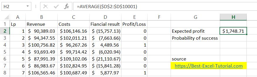
To calculate probability it is enough to sum column E. Excel Sum function will do the job.
The formula is =SUM($E$2:$E$10001)/10000
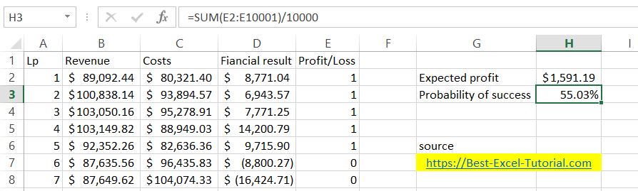
Hit F9 keyboard key several times. Please notice that the numbers change slightly. The more rows the smaller the changes will be.
Monte Carlo simulation is finished. Now, based on the number you can decide if it is worth to take the risk and introduce the product into the market. The simulation provides insights into the expected profit and the probability of making a profit.
Excel did the job, now it is on you to take a call.
You can download the free Monte Carlo simulation spreadsheet from here.


Leave a Reply