Search for string in column
In this article, you will teach yourself how to search for string in column. You may need this trick when you want to check if the cell contains string you need.
Table of Contents
Search for the string in cells
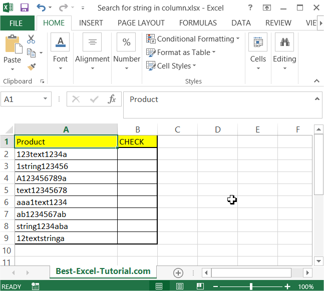
In this example you want to check if the cell contains either “text” or “string”. You will apply the formula to find string and substring in entire column.
In the data table below you see how data looks like.

To check if “text” or “string” exist just use this formula:
=IF(IFERROR(FIND(“text”,A2,1),0)+IFERROR(FIND(“string”,A2,1),0)>0,”TRUE”,”FALSE”)

This formula will display TRUE or FALSE in B column. No matter if it was a whole word or just a substring.
You can use conditional formatting if you want.
Using SEARCH and FIND
Both FIND and SEARCH locate the starting position of one text string within another.
- FIND (Case-Sensitive): =FIND(“text”,A2) finds “text” in A2, considering case. It returns the starting position if found, or a #VALUE! error if not.
- SEARCH (Case-Insensitive): =SEARCH(“text”,A2) is similar to FIND but ignores case.
To avoid #VALUE! errors, use IFERROR: =IFERROR(FIND(“text”,A2),”Not Found”). This returns “Not Found” if “text” isn’t found.
Using INDEX MATCH
Another method to search for a string within a column in Excel is to use the “INDEX” and “MATCH” functions together.
Here’s how you can use the “INDEX” and “MATCH” functions:
- Select the cell where you want to start the search.
- Type “=INDEX(” followed by the range of cells containing the data you want to search.
- Add a comma and enter “MATCH(” followed by the string you want to search for and a comma.
- Select the same range of cells as in step 2.
- Add a comma and enter “0” to indicate that you want an exact match.
- Close the parenthesis twice, and press Enter.
Here’s an example:
=INDEX(A2:A10,MATCH(“dog”,A2:A10,0))
This will search the range of cells from A2 to A10 for the string “dog”. If the string is found, the function will return the value in the same row from the first column of the range. If the string is not found, the function will return an #N/A error.
Like the “VLOOKUP” function, the “INDEX” and “MATCH” functions are also case-insensitive, so they will return the match even if the case of the string you’re searching for is different from the case in the cells.
Using FILTER function
Another method to search for a string within a column in Excel is to use the “FILTER” function.
Here’s how you can use the “FILTER” function:
- Select the cell where you want to start the search.
- Type “=FILTER(” followed by the range of cells containing the data you want to search.
- Add a comma and enter “,” followed by the string you want to search for.
- Close the parenthesis and press Enter.
Here’s an example:
=FILTER(A2:A10,”dog”)
This will search the range of cells from A2 to A10 for the string “dog”. If the string is found, the function will return an array of values that match the string. If the string is not found, the function will return an empty array.
Note that the “FILTER” function is case-sensitive, so it will only return the match if the case of the string you’re searching for is exactly the same as the case in the cells.
Extracting first/nth/last word from the string
Let’s see now how to extract the first, the nth or the last word from the string.
Suppose you have some string in A2 cell. You want to extract some part of this string. To do this you need to use formulas below.
To extract the first word from the string just use this formula:
=IFERROR(LEFT(A2,FIND(” “,A2)-1),””)
You may also extract the first word from the string with a leading space:
=IFERROR(LEFT(A2,FIND(” “,A2)),””)
This is a formula which let you extract the nth word. You string is A1 cell and the number of occurence is in B1.
=TRIM(RIGHT(SUBSTITUTE(LEFT(TRIM(A2),FIND(“^^”,SUBSTITUTE(TRIM(A2)&” “,” “,”^^”,B2))-1),” “,REPT(” “,100)),100))
And finally the last word you can extract with below Excel formula:
=IF(ISERR(FIND(” “,A2)),””,RIGHT(A2,LEN(A2)-FIND(“*”,SUBSTITUTE(A2,” “,”*”,LEN(A2)-LEN(SUBSTITUTE(A2,” “,””))))))
This guide has shown you several ways to search for strings in Excel, each with its strengths and weaknesses.


Leave a Reply