How to Create a Case-Sensitive VLOOKUP Formula in Excel
In this Excel lesson, you will teach yourself how to create a case-sensitive vlookup. This is a clever way to solve many problems caused by caps lock keyboard button.
Table of Contents
Case-sensitive vlookup
By default, VLOOKUP is not case sensitive, meaning that it treats uppercase and lowercase letters as the same. For example, if you use VLOOKUP to search for the value “apple” in a table that contains “Apple”, it will return the value in the same row.
Vlookup function doesn’t care about case-sensitivity. So what to do when you do?
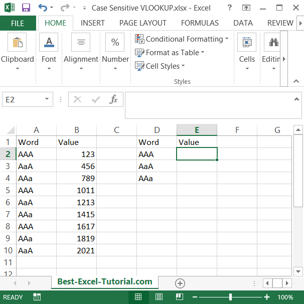
Here’s a practical case-sensitive VLOOKUP example with sample data:

The task is to vloookup the value to the word. Formula should care about case-sensitivity.
The solution is this array formula:
=VLOOKUP(value,IF(EXACT(value,column),table),column_number,0)
The parameter 0 forces the VLOOKUP function to search for an exact match only, which is essential when building case-sensitive lookup formulas.

Formula in the example is:
{=VLOOKUP($D2,IF(EXACT($D2,$A$2:$A$10),$A$2:$B$10),2;0)}
Please be aware that it is an array formula so you need to use CTRL + SHIFT + ENTER keyboard shortcut. That’s why there are braces around the formula. They appears after you typed CTRL + SHIFT + ENTER.
Keep in mind that this approach requires you to use additional columns and functions, which may not be as efficient as a simple VLOOKUP formula.
However, it gives you more control over the matching process and allows you to perform case-sensitive lookups when necessary.
Case-sensitive lookup
The problem is that your data differ only by case so capitalization is important for you. That’s why you need case sensitive lookup. Let’s construct a formula which will solve your problem. INDEX formula suits the best.
Syntax here will be:
=INDEX(value_you_need, row_number, column_number)
- value_you_need is a data range from your data table.
- row_number – this is hard to get. You have to use EXACT function for case sensitive function.
- column_number is always 1.
In this example you need the Price and you have Product IDs. The formula you need is:
=INDEX(B1:B5,SUMPRODUCT((EXACT(A1:A5,E2))*(ROW(A1:A5))),1)

Explanation:
- EXACT(A1:A5, E2): Returns TRUE for rows where the value in A1:A5 matches the value in E2 exactly (including case).
- ROW(A1:A5): Returns the row numbers of A1:A5.
- SUMPRODUCT(…): Multiplies TRUE values by their corresponding row numbers and sums them, effectively finding the exact match.
Choose the method that fits your needs, and remember to press CTRL + SHIFT + ENTER when entering array formulas.


Leave a Reply