How to Calculate Rolling Average in Excel
A rolling average is a type of moving average that calculates the average of a set of data points over a specified period. The period can be fixed or variable, and it is typically used to smooth out fluctuations in the data.
How to calculate a rolling average in Excel
There are two ways to calculate a rolling average in Excel: using formulas and using the Data Analysis ToolPak.
Using formulas
Using Average function
To calculate a rolling 6 months average in Excel, you can follow these steps:

Click on an empty cell, and type =AVERAGE($C$3:$C$3).

Click on cell D4, then write =AVERAGE($C$3:$C$4).

To copy the formula to the remaining cells, select the cell that contains the formula and drag the fill handle down to the last cell in the range.
The formula will be copied to the remaining cells and the rolling average will be calculated for each month.
Using INDEX function
Alternatively, you can use the INDEX function to select the range of cells:
- Select the cell where you want to display the rolling average.
- Enter the formula: =AVERAGE(INDEX(C:C,ROW()-n+1):INDEX(C:C,ROW())) Where:
- C:C is the column that contains your data.
- n is the number of data points you want to include in the rolling average.
For example, if you want to calculate a 6-month rolling average, the formula would be: =AVERAGE(INDEX(C:C,ROW()-5+1):INDEX(C:C,ROW()))
- Press Enter to calculate the rolling average for the first set of data.
- Copy the formula to the remaining cells in the column.
Note that the formulas will adjust automatically as you copy them to the rest of the cells in the column, and the rolling average will update accordingly.
kecyExege
Thank you for doing this