How to Highlight Every Other Row in Excel
In this tutorial, you’ll learn how to highlight every other row in Excel using conditional formatting for better data readability. Excel can automatically highlight alternate rows without manual coloring, saving time on large spreadsheets.
Setting conditional formatting rules
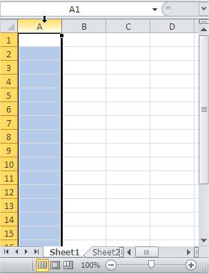
Start by selecting the Excel cell range where you want to apply alternate row shading.

To apply the alternating row highlighting, navigate to the Home tab on the ribbon and within the Styles group, select Conditional Formatting followed by New Rule…

In the New Formatting Rule dialog box, choose Use a formula to determine which cells to format.

Use the formula =MOD(ROW(),2)=1 to highlight odd-numbered rows in Excel using a formula-based rule. This formula checks if the row number is odd.

Click the Format… button to choose your desired formatting, such as a fill color, on the Fill tab of the Format Cells dialog box.

Applying this rule will highlight all odd-numbered rows within your selected range.
Highlighting Every Other Row
Cells are coloured. Conditional formatting started from first row.

To apply a different color to the even-numbered rows, repeat the process of creating a new conditional formatting rule, but this time use the formula =MOD(ROW(),2)=0.
This formula checks if the row number is even.

Choose a different formatting style, such as a contrasting fill color, to distinguish the even rows. This will result in alternating row colors across your selected range.

Tip1 – defining own conditional formatting
You can customize Excel’s conditional formatting with your own rules – apply colors, fonts, or borders to meet your visual needs. It can be also other kind of borders, colours, font style or pattern of cells. It’s your choice. Let’s prepare your custom conditional formatting like the ones I prepared:

Your new conditional formatting rule should now be applied to the selected range of cells in Excel. You can create multiple rules for different conditions by repeating these steps for each new rule that you want to define.
Tip2 – highlight every Nth row
You can also highlight every third of fourth row. Just change the number in formula.
Syntax for highlight every third row is =MOD(ROW(),3)=0 or =MOD(ROW(),3)=1 or =MOD(ROW(),3)=2, and the syntax for highlight every fourth row is =MOD(ROW(),4)=0 or =MOD(ROW(),4)=1 or =MOD(ROW(),4)=2 or =MOD(ROW(),4)=3.
Click on the Format button to choose the formatting that you want to apply. For example, you can select a background color for the cells that you want to highlight.

Your conditional formatting rule should now be applied to every Nth row in the selected range of cells in Excel. Note that you can replace N with any number you want to highlight rows at a different interval.
Using conditional formatting to highlight alternate rows improves data organization, making large Excel sheets easier to read and analyze. By using conditional formatting, you can quickly apply this formatting to a selected range of cells.
The steps to highlight every other row are simple and involve selecting the range of cells, choosing the Conditional Formatting option, creating a new rule using a formula, selecting a formatting option, and applying the rule to the range.


Leave a Reply