Excel has a set of pre-defined functions to perform various operations as desired. So, it is very easy to get to grips with a pre-defined function to execute any mathematical, statistical or logical operation. But there are certain circumstances where you need to deal with a custom or re-usable function in Excel.

You might think that you have to be an Excel ninja to create such a custom function that knows VBAs, Macros or JavaScript. But Excel has extended its capacity by letting any user with zero knowledge of programming define their own custom function with the help of the LAMBDA function.

Surprisingly, you can create a function that has similar characteristics to native Excel functions.

So, how do you use the Excel LAMBDA function? This is the ultimate guide for you to grasp everything you need to define your own function and use it in your spreadsheet as needed.

What is LAMBDA function

It’s common practice to use anonymous functions in some programming languages for a specific purpose, whereas using a built-in function is not efficient. But LAMBDA function in Excel makes you worry free to perform the said task for non-programmers like you.

However, it hasn’t got any mysterious mechanism which is hard to understand. Let’s dig in deep to discover what is LAMBDA all about.

LAMBDA function in Excel is a way of creating custom or reusable function to use throughout your workbook. You can simply give any name to this awesome function to make it unique.

LAMBDA functions can be typically simple or more complicated wrapped up of multiple built -in functions together.

Syntax

=LAMBDA ([parameter 1, parameter 2, …], calculation)

Arguments:

• Parameter: Optional. An input value that needs to be passed to the function. This can be a any form of data such as cell reference, string or number. You can add 253 parameters maximum.
• Calculation: Required. The formula that needs to executed. So, this returns the result of the defined function and thus, the last argument.

How do you create and use the LAMBDA function in Excel

Unlike native functions in Excel, custom functions are error-prone that outputs erroneous results. Because naturally you can make mistakes when creating custom functions.

Therefore, you can use formula bar in Excel to create and debug the function that you are going to create before use it in a LAMBDA function.

Let’s hop to an example to understand this better.

Example

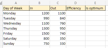
Suppose you are required to evaluate a machine’s overall performance in Excel in terms of its efficiency. You should check whether the machine is operating at its optimum level.

However, the problem has following breakdown for a better understanding of calculation.

• What is the machine’s efficiency?
• Is the machine operated at its optimum? (Machine’s min optimum value is 0.7)

First, you should properly understand and determine what are the inputs and output of the problem before building the main formula. Here are the inputs and output of this example.

Inputs: In and Out

Output: TRUE/ FALSE

Now let’s set up the main formula step-by-step to implement in LAMBDA function.

Step 1: Setting up main formula

First things first! You need to set up the main calculation or formula for this example accurately. In order to implement this in a LAMBDA function successfully, you need to build the logic for the above example in Excel spreadsheet.

Let’s complete above given criteria using Excel native functions and simple mathematical calculations.

Building the logic

What is the machine’s efficiency?

Machine’s efficiency = Out/ In

Machine’s efficiency with respect to cell references in Excel will look like this:

All efficiencies on Column D, will be calculated according to this form.

Is the machine operated at its optimum?

Given that machine’s minimum optimum value is 0.7, each efficiency should be compared to this value with the help of a conditional operator.

So that main formula will return true or false as the result of the comparison.

Is machine operated at its optimum = Efficiency > 0.7

Main formula with respect to cell references in Excel will look like this:

All records on Column E, will be calculated according to this form and will output TRUE or FALSE.

However, it’s vital to handle every possible error in this calculation in Excel. So that you won’t get confused on getting unexpected errors once the LAMBDA function is created.

Handling possible errors

Before jumping into handling errors, you need to assume what inputs would throw errors depending on the nature of your calculation.

Possible errors

Here are possible inputs that would throw errors:

In: Blank cell or 0

Because when the divisor is equal to blank to or 0 the formula will throw such an error in Excel.

You can use either IF or IFERROR functions depending on the output you are likely to have for this kind of situation.

So, we’ll move forward with returning 0 as the efficiency which is the simplest for the above inputs of “In”.

Correction

This is how to apply IF function for the no value or 0 inputs for “In”.

For no value inputs:

For 0 value inputs:

Now the main formula will return the result for above errors handled as shown below.

You can further test the formula for any possible errors in order to prevent unexpected behavior or errors once the LAMBDA function is set up.

Step 2: Creating the LAMDA function

Now you know the main formula requires inputs, so the parameters for the LAMBDA function. You should come up with two names for the two parameters. Make sure they reflect the same meaning same as the inputs’ name of main formula.

Let’s create the LAMBDA function and declare the parameters:

=LAMBDA (in, out)

Insert the function in main formula as the calculation of LAMBDA function. But you cannot use cell references in the original function. Instead replace them with corresponding parameter names:

=LAMBDA (in, out, IF (in, out/in,0) > 0.7)

Viola! You are done with creating the LAMBDA function. Now it’s important to test the created function with input values and Excel allows this with following notation:

=LAMBDA (in, out, IF (in, out/in,0) > 0.7) (function call)

Note: If you don’t use above formula without function call Excel will throw an error, “#CALC!”

As shown, result of the main formula for Monday will throw an error.

Here’s the tested result for Monday calling the LAMBDA function within the cell where the result needs to be shown. You need to pass two parameters same as the order defined in parameters declaration.

Make sure to include the parameters within the parentheses as shown below.

You will note that the result is appeared same as the result of original formula.

Step 3: Naming the LAMBDA function

Once you are happy with testing the LAMBDA function and found no issues you can move forward by naming your function.

The purpose of following this step is to register your LAMBDA function in Excel by providing it a name and description to make it re-usable and meaningful throughout your workbook.

Here are the steps to do it.

Select and copy the LAMDA formula without the functional call: 

=LAMBDA (in, out, IF (in, out/in,0) > 0.7)

Go to “Name Manager” either by pressing shortcut keys “Ctrl + F3” or by navigating:

Formulas > Name Manager.

Open “Name Manager” and click on “New”

In the popped-up dialog box fill each field as follows:

“Name”: A short but meaningful name to represent the main formula. In our example, formula is used to check the optimum efficiency value which is a condition. So, let’s name it “IsEfficiencyOptimum”.

Note: Make sure to follow naming rules in Excel to comply with its already defined rules

“Scope”: Keep the default value “Workbook” if you intend to use your defined formula throughout the workbook

“Refers to””: Paste the copied formula definition along with the equal sign at the beginning

If you are satisfied with the filled values to register the formula, click “OK” button. Your registered LAMBDA function will show up in a dialog box.

If you need to alter the formula definition you can edit it in “Refers to:” field and click on “Right” symbol.

Step 4: Using the defined LAMBDA function in Excel

Once you are done with registering your LAMBDA function, Excel lets you to utilize it like other native functions in Excel. New function’s name is “IsEfficiencyOptimum”, and you can now call it anywhere in the workbook just like other native functions.

So, let’s determine the result for “E2” cell using the new formula. You will notice the new function’s name is appeared in the dropdown once you start typing the function’s name in formula bar.

Now it’s a matter of selecting the function name and pass the arguments as required. You can provide “B2” and “C2” respectively for the arguments “in” and “out”.

Click “Enter” to get the result and you can drag the same application way down until “E8” cell.

Important usage notes of LAMBDA function

Even though you are allowed to define any function in Excel as you like, you must follow some standards in Excel and should know the limitations of usage.

Limitations of function usage

• You can utilize up to 253 parameters when defining a LAMBDA function and in case of exceeding the limit, it will throw #VALUE! error.
• Once you are using a defined function and passing incorrect number of parameters to the function, Excel will throw #VALUE! error.
• If you are calling your own created function within itself recursively, Excel will throw #NUM! error.

Function or parameter naming rules

• A name can only be 255 characters long
• You cannot add spaces in between characters or punctuation marks in the name
• First character of the name can be a letter, “_” (underscore) or “\” (backslash)
• Names are not case sensitive
• You are not allowed to use cell references or addresses as names in Excel
• You cannot use period (.) for parameter names

When to use LAMBDA function

Suppose you need copying and pasting same formula in multiple places throughout your workbook. You can simply eliminate lot of reworks by defining a LAMBDA function for the formula to make it reusable.

There’s another drawback entangled with the above situation. Assume you encountered an error in the function you used in multiple places. So, you need to correct every place that you applied the formula.

But using a LAMBDA function once to replace the formula, makes you alter the function once and it will get applied to all places where it is used.

Also, you can simply use LAMBDA function to create very simple formulas to quite complex ones which connects multiple native functions together in Excel.

When not to use LAMBDA function

Though this is an awesome function which allows you to create your own rules within a function just like other native function, there are certain situations where this function does not provide its value to the fullest.

When you have lot of customizations between formulas that you use in your workbook it is not ideal to use LAMBDA function to create a custom function to each one of them.

Note: You can download this Excel tutorial file which includes the example explained in this tutorial by clicking here.