In this lesson, you can learn how to use filters in Excel.

Excel has a feature of filters that make it easy to find the data you need in your spreadsheets. Filters allow you to view and optionally print only selected data from the table, and perform mathematical operations, taking only the visible data.

We will show you how to use filters in Excel. We will start by explaining the different types of filters available in Excel, and then we will show you how to use them to filter data in a table.

Types of Filters in Excel

There are two main types of filters in Excel: automatic filters and advanced filters.

• Auto Filter, the most frequently used filtering method, allows you to quickly filter data based on the values within a single column. For example, you could use Auto Filter to display only products belonging to “Category1”.
• Advanced Filter offers more sophisticated filtering capabilities, enabling you to filter based on multiple criteria across different columns. For instance, you could use Advanced Filter to display only products that are in “Category1” and have a price less than $100.

How to Use Filters in Excel

To use filters in Excel, you first need to select the range of cells that you want to filter. Then, you can use the following steps:

1. Click on the Data tab.
2. In the Sort & Filter group, click on the Filter button.
3. A drop-down menu will appear. Select the type of filter that you want to use.
4. The filtered data will be displayed in the table.

Example – easy filtering by category in Excel

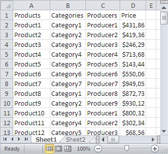
For example, let’s apply filters to a table of products to narrow down the selection by category.

Select the table header row.

Go to the Ribbon. In the Home tab, click the Sort & Filter icon and select Filter from the list.

In the table appeared some buttons to filter the data.

Click on the Categories. In the list, uncheck the category which you want to be hidden (filtered), such as Category2.

After applying a filter, you can’t see products from Category2.

On the picture above, you can also see that some rows are hidden. You don’t see 3 and 10 row. In the B1 cell, you can also see a symbol of filter close to the arrow. That means that this column is filtered.

If you want to filter more, you can. Let’s hide products from Producer3 and Producer5.

You can also filter prices. There’s number filters. Click filter arrow in D1 cell.

I want to find the cheapest. I select Less Than Or Equal To.

My budget is $150.

That’s how I filtered out products which I don’t want in my table.

Now it is much easier to choose one.

Clearing Filters: Removing Restrictions

To remove the filter from a single column, click its filter arrow and select “All” (which checks all values) or use a “Show All” option if visible. Unchecking all values in a filter does the opposite—it hides everything in that column, leaving only the header visible. That’s rarely what you want, but it’s technically possible.

To remove all filters at once and display every row again, click Data and select Clear. This removes all active filters while keeping the filter arrows in place, so you can easily reapply filters later. To completely remove AutoFilter (hiding the filter arrows), click the Filter button in the Data tab again to toggle AutoFilter off, or press Ctrl+Shift+L.

Some users accidentally apply filters then forget they’re active. They later wonder why certain data isn’t visible or why totals don’t match expectations. Checking the row numbers and status bar is your diagnostic tool. If row numbers jump (like 1-10, then 15-25, skipping 11-14), filtering is active. The status bar shows “X of Y records” when filtering is active, confirming your suspicion.

Practical Filtering Scenarios

Picture a sales spreadsheet with hundreds of transactions across months. Your manager asks, “How many deals closed in September worth over $50,000?” Filter the Month column to show only September. Filter the Amount column to show only values above 50,000. Filter the Status column to show only “Closed.” Now the visible rows are exactly what you need. Count them manually or create a SUBTOTAL formula to count visible rows. Done in seconds.

Or you’re managing a project with dozens of tasks. Some are assigned to you, some to colleagues, some unassigned. You want to see only your tasks. Filter the Assigned To column to show only your name. Now you see just your tasks, their status, due dates, and priorities. You can sort this filtered view by due date to see your work in order of urgency. Remove the filter when you
want to see everything again.

Another common scenario: customer service analyzing complaints. You have 1,000 tickets. You want to see only tickets from the last month (filter Date) that have priority “High” (filter Priority) and status “Unresolved” (filter Status). These three filters create a focused view of urgent work. You might sort by date within this filtered view to handle oldest first. This combination of filtering and sorting is how professionals manage complex data.

Copying and Pasting Filtered Data

A subtle but important behavior: when you copy filtered data, Excel copies only the visible rows by default. If you select a range that includes hidden rows, copy, and paste, the paste operation includes only visible cells. This is usually what you want—you’ve filtered to see specific data and you want to copy just that subset. The hidden rows stay hidden and don’t get copied.

Conversely, if you accidentally copy without realizing filtering is active, you might copy less data than you intended. It’s worth checking for active filters before large copy operations. Look at the row numbers and status bar to confirm you’re not filtering unknowingly.

Pasting into a filtered range is trickier. Generally, avoid it because Excel gets confused about where to put pasted data when rows are hidden. If you need to paste, first remove all filters, paste your data, then reapply filters. This avoids unexpected placement or overwriting of hidden data.

Once you’re comfortable filtering, learn sorting to complete your data organization toolkit. Explore how to create basic charts from filtered data to visualize your focused analysis. Then discover Excel tables for enhanced filtering with automatic formatting and expanded capabilities.

Practical Applications in Business: Next Steps

Now that you understand the fundamental concepts of this Excel feature, the next logical step is to apply them to real-world business scenarios and advanced analysis. Our comprehensive learning hubs show how professionals use these foundations to build dashboards, analyze data, and make strategic decisions.

These hubs bridge the gap between Excel basics and professional applications. Start with the hub that matches your role or goals—each provides step-by-step guidance and real-world examples.

Related posts:

11 Best Excel Add-ins to Boost Productivity Understanding Excel Cells, Rows and Columns: The Foundation of Everything Copy and Paste in Excel: Master Every Technique from Basic to Advanced