Chart with combo box
In this Excel tutorial, you will learn how to insert chart with combo box.
Table of Contents
Adding a combo box for a chart
Prepare a table of data.

Copy and paste a list of arguments (countries in my example) to another column. You will need it soon.

Go to the ribbon to the Developer tab. Insert a combo box using VBA controls.

Right-click your combo box and select Format Control.

Set Properties of your combobox. Input range are your values from the list you created at the beginning. Set also a Cell link wherever you want.

Cell link is here. There will be a velue you will need for your chart.

Combo box works since here. You can try it out. In the cell link there will be a value 1 – 4. It depends on country you will choose.
Copy first column of your table and paste it below.

In B column header (B16 in my example) write this formula: =INDEX(list_of_countries, cell_link). In my example it is =INDEX(P3:P6;B14)
In B17 write another formula down. It is =VLOOKUP(product_name, data_table, cell_link + 1, FALSE). Here it is =VLOOKUP(A17;$A$3:$E$12;$B$14+1;FALSE)
Next drag and drop this formula down. This way you created a new table with same data such in table.

Creating a combo box chart
Almost everything is done. Next, you will create a chart.
Highlight your table with sales data but only A and B column.

Go to the ribbon and create a column chart. This is how it looks like.

Your combo box works. Go there and change a value from drop-down list. Your chart will change like mine here.

Finally, your chart with a combo box is ready.
Leave a Reply