3D clustered column charts are a great way to visualize data in Excel. They are easy to create and can be used to compare multiple data series. In this article, we will learn how to create a 3D clustered column chart in Excel.

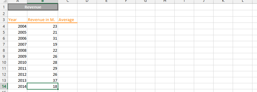
Data preparation

Before creating a 3D clustered column chart, you need to prepare your data. Your data should be in a column format, with the labels in the first column and the values in the subsequent columns.

Select the data that you want to chart.

Creating 3D Clustered Column Chart

Click on the Insert tab.

In the Charts group, click on the Column chart type.

Select the 3-D Clustered Column chart subtype.

In conclusion, we have just created a 3-D chart that looks like this:

Formatting the chart

Once you have created the chart, you can format it to your liking. You can change the chart title, axis labels, gridlines, and data labels. You can also change the color scheme, font size, and other elements of the chart’s appearance.

Adding data series

If you want to include multiple data series in the same chart, repeat steps 1-4 for each additional data set. You can then select the chart, go to the Design tab, and click on Select Data. Add the additional data series to the chart by clicking Add and selecting the range for each series.

Adjusting 3D formatting

You can adjust the 3D formatting of the chart by right-clicking on the chart and selecting Format Data Series. In the Format Data Series pane, click on the 3-D Format tab. Here, you can adjust the depth of the chart, the angle of view, and other 3D elements.

Adding a secondary axis

A secondary axis can be used to plot a different type of data on the same chart as your primary data. This can be useful for comparing two different types of data that are on different scales.

To add a secondary axis to your 3D clustered column chart, follow these steps:

1. Right-click on one of the data series in the chart and select Format Data Series.
2. In the Format Data Series pane, click on the Axis tab.
3. Under the Vertical axis section, select Secondary axis.

Excel will add a secondary axis to the chart. You can then plot your secondary data on the secondary axis by following the same steps you used to plot your primary data.

Adding error bars

Error bars can be used to show the variability of your data. This can be useful for showing the margin of error for your data points or for comparing the variability of different data series.

To add error bars to your 3D clustered column chart, follow these steps:

1. Right-click on one of the data series in the chart and select Format Data Series.
2. In the Format Data Series pane, click on the Error Bars tab.
3. Select the type of error bars that you want to add and enter the appropriate values.

Excel will add error bars to the chart. You can then customize the appearance of the error bars by clicking on the Format Error Bars button.

Finalizing the chart

Once you have formatted the chart to your liking, you can save it or insert it into your Excel workbook. You can also use the chart in other applications, such as Word or PowerPoint, by copying and pasting it into the desired location.

You can download free 3D chart template here

Related posts:

How to Make a Pareto Chart in Excel How to Make a Pie chart Time Series Graph