In this lesson, you will learn how to sort data in Excel. Sorting data can help you make your spreadsheets more organized and easier to read. It can also help you identify patterns and trends in your data.

Sorting in Excel

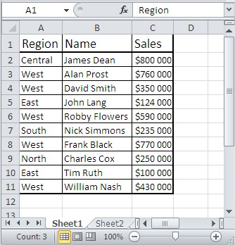
To sort data in Excel, you first need to select the data you want to sort. In the example below, we want to sort the data in the range A1:C11.

Once you’ve selected the data (e.g., A1:C11), go to the Data tab and click the Sort button.

In the Sort dialog box, you can choose the column you want to sort by, and the order you want to sort it in. We want to sort the data by the Sales column in descending order.

You can also add another sort level by clicking on the Add Level button. This will allow you to sort the data by another column, such as the Region column.

Now your data is sorted, making it easier to analyze or present.

Download sample spreadsheet for free.

How to sort by more than three columns?

It is easy to sort more than three columns.

Click on the first data cell.

Click Data and then press Sort.

Sort by “Year of Employment”.

Repeat, but in the sort criteria, select the manager (or the most important column) and then click Add Level to select the second most important column.

Note that you need to repeat this step until you have sorted the columns from most important to least important. If the cells in the column change positions for the sort to take effect, Excel ignores them.

Sorting by color

You can also sort the colors. You may need this feature if you like to colorize your spreadsheets.

To sort the colors in the table, first prepare a colored data table like the one in the picture below.

Click Data and then click Sort.

Select a column and then select a color to sort by. Finally, select the order.

Note that after completing this step, you need to click the Add Level button, sort by the same column, and select the color you want second. Continue this process until you have added all the colors in your data.

How to Sort by Row?

Did you know that you can also sort by rows? This trick can be useful for large spreadsheets with multiple columns.

First, prepare a data table.

Go to the ribbon on the Data tab. Click the Sort button.

Click the Options button.

You’ll see a choice between “Sort top to bottom” (the default) and “Sort left to right”. Select “Sort left to right” and now the dialog changes perspective.

Instead of choosing which column to sort by, you choose which row. If row 7 contains the totals for each month and you want columns arranged from highest to lowest total, select
row 7 and set the order to largest to smallest.

When you click OK, the columns rearrange themselves. The column with the highest total moves leftmost, the next highest moves beside it, and so on. All the rows in each column move together, so the data integrity remains perfect. This type of sort is less common but when you need it, it’s invaluable.

Sort the word list by the number of characters

Excel can sort data in a variety of ways. You can also sort data by the number of characters.

In column B, type the formula =LEN(A2).

Drag the formula down to the rest of the cells in column B.

Now you can see the character count of the word from column A in column B.

Then select the entire table. On the ribbon, go to the Data tab. In the Sort dialog box, check the My data has headers box and select Number of characters from the Sort by drop-down list. Select Smallest to largest from the Order drop-down list.

Excel sorts words from the shortest to the longest.

After sorting, you can hide the helper column if you don’t want it visible. Right-click the column letter and choose Hide. The column still exists and maintains your sort order, but viewers won’t see the calculated values you used for sorting.

How to Sort Out Blank Rows?

Sorting out blank rows depends on how many there are and whether they should be there or not. First, look at these lines that have both filled and blank cells:

To find all blank rows quickly, select your entire data range.

Press Ctrl+G to open the Go To dialog. Click the Special button.

Select Blanks.

On the Home tab, select a color from the Cell Styles menu.

Select all data again.

Click Data (1) and then Sort (2).

Select a category to Sort by, select a cell color in Sort on, No cell color in the order, On top.

Select all colored lines, right-click the selected lines and select Delete.

How to sort whole worksheet by one column?

Whether you have a simple dataset or a large datasheet, sorting is a simple and effective way to organize and analyze your data in Excel. You can sort data by a variety of options, including the built-in filtering feature and custom sorts.

Regardless of the number of columns, rows, and cells in a worksheet, you can sort the entire worksheet by one column in seconds. Let’s see how you can sort whole worksheet by one column in Excel.

To sort your data, you need to organize it into rows and columns. You will also need dedicated column headers as this will make it easier to sort your data. Select the row that contains the column headings or drag and select all the column headings to start sorting.

After selecting the column headings, select Data> Filter – this will add drop-down icons to the column headings.

Simply select the column you want to sort by. In the drop-down menu, you will see the available sorting options, which depend on the data in the selected column. For columns that contain numbers, you can choose to sort from largest to smallest, smallest to greatest, or you can set a custom sort.

By selecting one of the sort options, you will sort the entire sheet based on that one column. All data in the other columns will also be sorted.

If you also select a text column, Excel will allow you to sort A to Z, Z to A, or according to a custom sort option you enter. Sorting an entire worksheet by one column is a simple and effective way to organize your data.