In this Excel tutorial, you will learn how to create a formula which returns the last value in a column.

This tutorial is useful when you have a column of data and sometimes you add some data there. In this case you can easy to return the last value to some cell you want.

The Index Match formula to get the last value

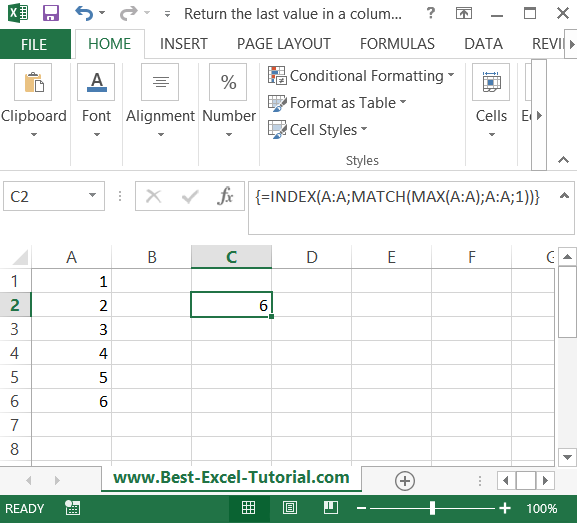
Use the INDEX MATCH functions combinations for that purpose. To return the last value from the last cell in the A column just use this Excel formula: =INDEX(A:A;MATCH(MAX(A:A);A:A;1))

This is an array formula so to execute it you should use this keyboard keys: CTRL + SHIFT + ENTER.

Tip: This formula also works when you have some empty cells in the column.

The Lookup formula to get the last value

This method uses the LOOKUP function to return the last value in a column. The LOOKUP function returns the last value in a range that matches a specified value. Here’s how to use this method:

• Enter the following formula into a cell: =LOOKUP(2,1/(A1:A100<>””),A1:A100)
• Replace A1:A100 with the range that contains the column you want to retrieve the last value from.
• The formula creates an array of 1s and 0s that corresponds to the cells in the range. The 1s correspond to non-empty cells, and the 0s correspond to empty cells.
• The LOOKUP function then searches for the last 1 in the array and returns the value in the corresponding cell in the range.

The Index Match formula to get the last value

This method uses the MAX function to return the last value in a column. The MAX function returns the largest value in a range. Here’s how to use this method:

• Enter the following formula into a cell: =MAX(A1:A100)
• Replace A1:A100 with the range that contains the column you want to retrieve the last value from.
• The MAX function returns the largest value in the range, which is the last value in the column if the values are sorted in ascending order.

Related posts:

How to Get Data from another Sheet? Time in milliseconds in Excel How to Sum only Positive / Negative Numbers in Excel