How to calculate covariance in Excel?
In this Excel tutorial, you will learn how to calculate covariance in Excel.
We can detect the existence of a correlation by examining the covariance.
Covariance is the average of the products of the deviations of each data point pair.
Use covariance to define the relationship between two datasets.
- A positive value of covariance occurs when both variables are moving in the same direction.
- Negative covariance occurs when an increase in the value of one feature tends to decrease the value of the other.
- It is also possible that the covariance is zero. This means that the variables are not correlated.
Table of Contents
Sample Covariance
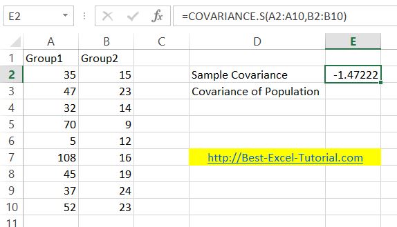
To calculate sample covariance use the COVARIANCE.S Excel function.
COVARIANCE.S syntax
=COVARIANCE.S(array1, array2)
In the given example, sample covariance formula is =COVARIANCE.S(A2:A10,B2:B10)

Population Covariance
To calculate population covariance use the COVARIANCE.P Excel function.
COVARIANCE.P syntax
=COVARIANCE.S(array1,array2)
In the given example population covariance formula is =COVARIANCE.P(A2:A10,B2:B10)

In most cases, you will use sample covariance. Use covariance of population function only when it is specifically stated that it is population covariance.
Using the Data analysis tool
Using functions to calculate the covariance is effective. I prefer to use the data analysis tool for covariance calculation. It is also a convenient way to calculate the covariance of a data table. Excel will prepare a covariance report based on the values you provide.
To calculate the covariance with the data analysis tool, first go to the Excel ribbon. Click the Data tab. On the right side you will find the Data Analysis button.

A window will appear. Select Covariance from the menu.
In the next window, determine the input range. The covariance input is your entire data table. If you also select the row with headings, then check the Labels in first row option.

Select the place where you want the result to appear as the output range. If you have free space on the worksheet, enter the cell address. Otherwise, check New Worksheet Ply.
The covariance report will appear in the position you selected as output in the previous window.

Download a covariance calculator here.
It’s important to note that the covariance value alone doesn’t fully explain the relationship between two variables. Other statistical measures are also important. The correlation coefficient shows the strength and direction of the linear relationship. The coefficient of determination shows how much of one variable’s variation is explained by the other.
For a better understanding of the relationship, check the correlation coefficient with =CORREL(array1, array2).


Leave a Reply