In this Excel tutorial, you’ll learn how to transform a static chart into a dynamic chart that updates automatically based on your data. Dynamic charts in Excel are useful when you need charts that update automatically when your data changes or expands.

People who can make dynamic charts in Excel are truly Excel’s experts. Become one of them and learn how to create dynamic charts.

There are two ways to create dynamic charts in Excel.

Example 1 Create a Dynamic Chart in Excel That Responds to Cell Input

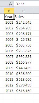
First, prepare a data table in Excel, such as yearly sales figures.

Create a simple column chart from your static data—this will become your dynamic Excel chart.

Next, go to Ribbon > Formulas > Define name. Define B and C column as Year and Sales.

For the Year range, use this OFFSET formula: =OFFSET(Sheet1!$B$2,0,0,Sheet1!$A$1,1)—this lets you dynamically control how many years appear based on the value in A1.

For the “Sales” data (starting in C2), use =OFFSET(Sheet1!$C$2,0,0,Sheet1!$A$1,1)

Cell A1 will control the number of rows included in the chart. Then, right-click the chart, select Select Data.

Edit the series. If there is only one serie – Sales but you can have more.

Series name is: =Sheet1!$C$1

Sheet1 is the name of my sheet.

C1 is the cell where I have my Sales serie.

Series values are: =‘Dynamic chart.xlsx’!Sales

Dynamic chart is the name of my spreadsheet.

Sales is the name which I defined.

Now, the chart becomes dynamic. You created dynamic chart which works really easy way.

Now, when you enter a number into cell A1, your Excel chart will update to show that many years of data.

There is an example for 13 years.

The is an example for only 6 years.

As you see chart changes. On the chart there are only as many years as you wrote in A1 cell before.

You can also start from the newest year. Just change formulas from:

=OFFSET(Sheet1!$B$2,0,Sheet1!$A$1) for Year

=OFFSET(Sheet1!$C$2,0,Sheet1!$A$1) for Sales

to:

=OFFSET(Sheet1!$B$14,0,Sheet1!$A$1) for Year

=OFFSET(Sheet1!$C$14,0,Sheet1!$A$1) for Sales

Now, write some values into A1 cell with minus sign. That’s how it looks like for 6 years and 8 years.

Chart changes really good. Isn’t it amazing?

Example 2 How to Create an Auto-Expanding Dynamic Chart in Excel

Another way to create a dynamic chart is to have it automatically expand its data range when new data is added to the source table. This method is ideal for Excel sheets where new data is added frequently. Use COUNTA and OFFSET together to create dynamic named ranges that automatically grow as new data is added. For Sales, use =OFFSET(Sheet1!$C$2,COUNTA(Sheet1!$C:$C)-1)

For Year, use =OFFSET(Sheet1!$B$2,COUNTA(Sheet1!$C:$C)-1)

The COUNTA function dynamically counts the number of entries in the specified column, automatically adjusting the named range and, consequently, the chart’s data source, as new data is entered.

Now, your auto-updating dynamic chart is ready—it will expand automatically every time you add new data.

Dynamic charts are among the most powerful tools in Excel for real-time data visualization. It works really good and proves that you are Excel’s PRO.

You can download a free dynamic template from this link.

Related posts:

How to Create a Histogram in Excel How to Make a Pareto Chart in Excel How to Make Gauss Normal Distribution Chart