How to create IN and OUT Inventory System in Excel?
Excel is a great software if you want to take your inventory system or management forward. It’s a great tool for small businesses that automates processes that are usually done by hand.
Good thing about it is that Excel’s files can be opened with other accounting software, it’s files can be converted without much effort.
It’s much more effective than accounting on paper, because Excel has a variety of functions and tools that ease up the whole process. You will have a clearer view into your finances, budget and items.
It’s a great option if you are on a budget, it’s affordable and for it’s price you are going to get a perfect device for tracking down your expenses, items, decisions and everything else.
It will help you decide:
- Which items you need,
- What you should sell,
- Which price to set,
- What to restock,
- How to calculate GST or VAT,
This article will teach you how to make your own inventory system in Excel, whether you are an individual or a small corporation.
Table of Contents
How to begin?
The great thing about Excel is that most of the important things are not done by hand, but instead automatically with the features and tools that Excel includes.
Instead of manually creating a table and deciding what to put in and out. Excel allows you to look up pre-made templates that you can use in your spreadsheet.
Here is the step by step process on how to find a template in Excel:
- Click on the File button that’s on the top left corner,
- Then click New
- And from there you will have a variety of templates which you can choose from,
- Select inventories because that’s what you are looking for,
- You’ll then have access to a big number of inventory templates that can suit your needs.
This is a template that we chose as an example so you can see how it actually looks and works.
It is a regular inventory list, where you can see:
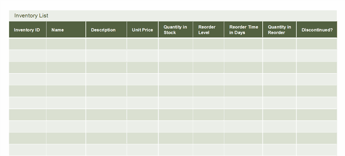
- Inventory ID – This is a unique ID that every product has, it’s used for identification of the said product. Instead of filling everything manually you can fill it automatically by selecting Fill Series when pulling down, or double clicking, a black cube that appears when you select a cell.
- Name and Description – These are pretty self explanatory, just input product names and description so you can recognize what’s what,
- Unit Price – When you select a cell, under Home you can find a Number section, where when you click on a dollar symbol you activate Accounting Number Format, which formats the number from the selected cell into a currency,
- Quantity in Stock – Enter the number of how many products you have left in the stock.
- Reorder Level – This is a minimal number of units that you must have in stock before you consider it low,
- Reorder Time In Days – This measures how long it will take you to get your items relinquished,
- Quantity in Reorder – This is the number of items you have reordered,
- Discontinued – This is the number of items that have been discontinued.
As you can see, navigating an inventory can be pretty simple when done in a software that has everything organized for you.
Functions
Excel is full of useful functions that make your accounting easier.
One of the unique and most important features it has are formulas. They are what makes Excel stand out, and we are going to pass by some important formulas that you are going to be using during your accounting in Excel.
They are:
- SUM – This formula calculates all values in the selected cells,
- AVERAGE – This formula gives you an average value of selected cells,
- IF – This formula gives you an opportunity to create if scenarios, for example if the value is higher than a certain number, a certain action should happen,
- VLOOKUP and HLOOKUP – These two formulas let you search a certain value in a table array, so they can return a value from a different column in the same row.
- There is also AutoSum, which automatically selects the cells that you want to calculate. It is not a formula but an option which can be found in the Formula section. It is useful if you are going to have to calculate a lot.
- One of the functions that you can use is Sort. You activate it by right clicking on the selected cell, then by clicking on Sort you will have a number of options for filtering things, like from A to Z, or Z to A, from largest to lowest, etc.

Leave a Reply