How to create many-to-many lookup in Excel
In Excel, you can perform a many-to-many lookup to find multiple values based on a single criterion. This is useful for tasks such as finding all the books that a certain author has written for a specific publisher, or all the products that a certain customer has bought from a specific store.
We will show you how to perform a many-to-many lookup in Excel using different functions and formulas.
Table of Contents
What is a Many-to-Many Lookup?
A many-to-many lookup is a type of lookup where you have more than one value in both the lookup column and the return column.
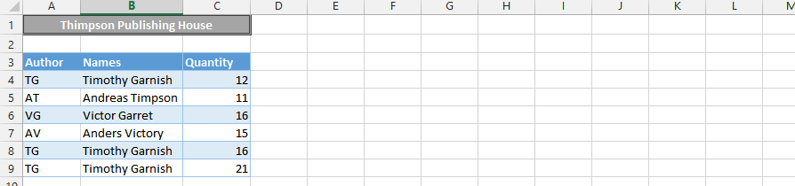
For example, in the table below, we have a list of authors, publishers, and books. Each author can write multiple books for multiple publishers, and each publisher can publish multiple books by multiple authors. This is a many-to-many relationship.
If we want to look up all the books that the author has written for the publisher, we cannot use a simple VLOOKUP or INDEX-MATCH formula, because they can only return one value per lookup.
We need a formula that can return multiple values for a single lookup value. This is where a many-to-many lookup comes in handy.
How to Perform a Many-to-Many Lookup in Excel?
There are different ways to perform a many-to-many lookup in Excel, but one of the most common and versatile methods is to use a combination of SUMPRODUCT, INDEX, SMALL, IF, ISNUMBER, ROW, and ROWS functions.
Prepare the data
The first step is to prepare your data in a table format, with headers and no blank rows or columns. Make sure that your lookup column and return column have unique values, or at least no duplicates within the same row.

Count the Number of Matches
The next step is to count how many matches there are for your lookup value. Lay out what you are looking for; in this case, I am looking for Timothy Garnish, who is also TG.

To do this, we can use the SUMPRODUCT function, which multiplies corresponding elements in two or more arrays and returns the sum of the products.
Type in this formula =SUMPRODUCT((B4:B9=B11)*(A4:A9=B12)*(C4:C9))

We just looked up the sum of all books that Timothy Garnish has written for the Thimpson Publishing House, as it is showing above.
How to return many items for a single lookup value?
There are different ways to return many items for a single lookup value in Excel.
We are going to use COUNT function in one single formula to find many items.

Type in =COUNT(A4:A10) in the formula box.

The lookup formula
If you prefer a formula-based approach and are not using Excel 365, you can use an array formula with INDEX, SMALL, IF, and ROW functions.
Type =IF(ROWS(C$2:C2)<=$B$2,INDEX($A$2:$A$10,SMALL(IF(ISNUMBER($A$2:$A$10),ROW($A$2:$A$10)-ROW($A$2)+1), ROWS(C$2:C2))),””) and then press F2.
Now press CTRL + SHIFT + ENTER as it is an array function.

In modern versions of Excel (Excel 365 and later), the FILTER function provides a much simpler and more efficient way to perform many-to-many lookups.
For example, to retrieve all books by “Timothy Garnish” published by “Thimpson Publishing House”, you could use a formula like =FILTER(BookRange,(AuthorRange=”Timothy Garnish”)*(PublisherRange=”Thimpson Publishing House”)), where BookRange, AuthorRange, and PublisherRange are named ranges.
For older versions of Excel or for more complex data transformations, Power Query (Get & Transform Data) offers a powerful and flexible solution.


Leave a Reply