Apply a Formula to an Entire Column in Excel: 5 Methods Explained
In this article, you will learn how to copy a formula into every cell in a column or row.
Table of Contents
Drag and Drop
Copying values in tables is easy. Take a look at the picture below. You should only put the cursor at the right bottom of the cell and double-click.

Values are inserted only in the cells that have neighboring cells with data.

Double-click
Another option is more convenient. This is a good choice for large data sets when drag and drop way is not an option.
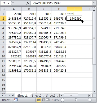
Start by positioning the cursor over the bottom-right corner of the cell. Your cursor should look like in the picture below.
The difference is that instead of dragging you need to double-click this corner.
Excel applied the formula to the entire column. It is alligning to the column in the left hand side. You can see that Column D contains the data until the row number thirteen. This is exactly where Excel will reach the same in the Column E.
Fill down
But what to do when you want to copy an entire column or row? There is a Fill option in the Ribbon in Excel.

Put your formula in the first row of the entire column. Select the whole column and use Fill > Down column.

This automated spreadsheet formula application technique successfully fills all cells throughout the column. The remaining empty rows below represent areas where adjacent data wasn’t available, ensuring your automated spreadsheet formula application remains efficient and accurate.

You can also copy an entire row the same way. Use Fill > Right then instead Fill > Down.
When implementing efficient Excel formula extension methods, the system automatically extends operations to all cells in the data range until reaching the final occupied position. For precise control over efficient Excel formula extension methods on selected cells only, you can manually specify the target range before initiating the fill operation.
Using Excel Tables
Excel Tables, also known as ListObjects, are a powerful feature that simplifies working with data. They automatically expand to include new data and allow you to apply formulas efficiently. Here’s how to use them:
- Select your dataset, including the column where you want to apply the formula.
- Go to the “Insert” tab and choose “Table” or press Ctrl + T.
- Ensure the “My table has headers” option is selected if your data has headers.
Now, you have a structured Excel Table, and any formula you apply in a column is automatically extended as new data is added below. Excel handles this expansion dynamically.
Using Excel Tables with Structured References
Structured references are a feature of Excel Tables that allow you to refer to table columns in a more readable and dynamic way. You can use them in formulas to apply calculations across entire columns. Here’s how:
- Assume you have a table named “SalesData” with columns “Product” and “Revenue”.
- To calculate the total revenue for all products, enter the formula =SUM(SalesData[Revenue]) in a cell outside the table.
This formula uses structured references to refer to the “Revenue” column in the “SalesData” table. As new data is added to the table, the formula updates automatically.
Using Defined Names
Another advanced method involves using Defined Names (also known as Named Ranges) to apply formulas to entire columns. Here’s how to set it up:
- Select the entire column where you want to apply the formula.
- In the “Formulas” tab, click “Define Name” or press Ctrl + F3.
- Give the name a descriptive title, like “TotalRevenue”.
- In the “Refers to” field, enter your formula. For example, =SUM(Sheet1!$B$2:INDEX(Sheet1!$B:$B,COUNTA(Sheet1!$B:$B))).
Now, you can use the defined name, “TotalRevenue”, in your formulas. It will automatically adjust to accommodate new data added to the column.
Using Dynamic Array Formulas
You can leverage dynamic array formulas to apply calculations to entire columns without worrying about the exact number of rows. For example, to calculate the total revenue for all products in a column:
In a cell, enter the formula =SUM(SalesData[Revenue]).
Excel will automatically spill the result over multiple cells below the formula, covering all the relevant data in the column.
These methods ensure that your calculations remain accurate and dynamic, even as your data grows or changes. Choose the approach that best suits your specific needs to work more efficiently with your data.


Leave a Reply