How To Use The Index And Match Functions In Excel
There are many functions in Excel that are useful in a variety of situations. Two of the most popular functions in Excel are the INDEX and MATCH functions. These functions can be used to look up values in a table or range of cells. Understanding these functions gives you the tools to make your data work for you.
In this Excel tutorial, we’ll show you how to use the INDEX and MATCH functions to get the most out of your data. We’ll also provide some tips on when these functions can be particularly useful. So, if you’re ready to learn more about these handy little functions, read on!
What Are The Benefits Of Using INDEX And MATCH Functions?
Together, these functions can be used to lookup values in a table or range. For example, you can use them to find the product ID for a given product name or the customer ID for a given customer name.
There are several benefits to using the INDEX and MATCH functions:
-
- Firstly, They are very versatile and can be used for a variety of tasks.
- Secondly, They are easy to learn and use.
- Thirdly, They can save you time and effort when looking up values in a table or range.
- Finally, Faster and less intensive on your computer than the VLOOKUP function.
Understanding The INDEX And MATCH Functions
To use the INDEX and MATCH functions, you will need to understand how each function works.
The INDEX Function
The INDEX function returns the value at a given position in a range or array. The syntax for the INDEX function is:
INDEX(array, row_num, column _num)
Specifically, The array is the range that contains the values you want to search for. This refers to the cells of the table, excluding the header row. The row_num is the row number that you want to return a value from. The column_num is the column number that you want to return a value from.
Additionally, You can use the INDEX function to return a single value or multiple values.
Using The INDEX Function On A Single Value
If you want to return a single value, you will need to specify the row_num and column_num for the value that you want to return. For example, to return the value in the first row and first column of a range, use:
=INDEX(range, 1, 1)
Practice – INDEX Function On A Single Value
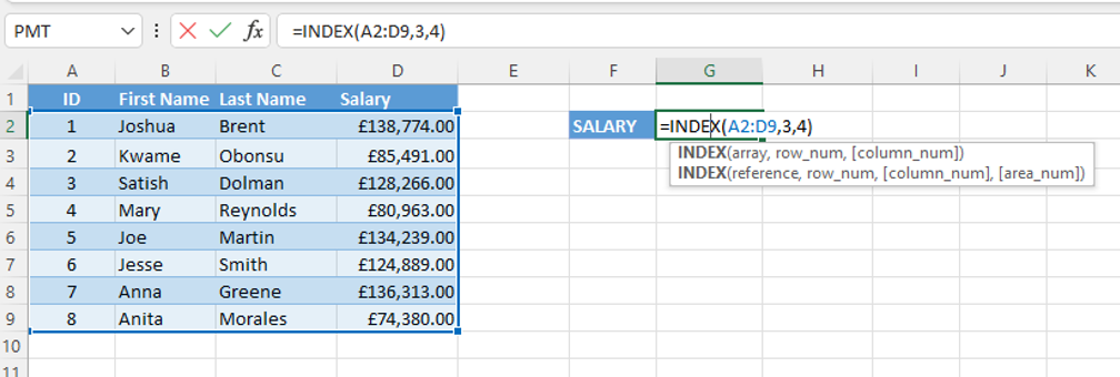
We have sample data for use throughout this article for you to use for practice. For instance, In this example, we have a list of employees and their salaries and want to return the salary for Satish.
Details we need:
- Array – A2:D9
- Row – 3 (excluding the title row)
- Column – 4
- Formula – =INDEX(A2:D9,3,4)
Open a spreadsheet How to use the INDEX and MATCH functions in Excel.xlsx, Index tab.
Click in G2, enter =INDEX(A2:D9,3,4)

Excel returns the salary of £128,266.00.

Overall, The INDEX function looks simple at this stage, but when combined with the MATCH function, as you’ll see later, it can provide a dynamic lookup tool for your data.
Practice – INDEX Function On Multiple Values – Column
Alternatively, If you want to return multiple values, you can leave the row_num or column_num blank. For example, to return all the values in the first column of a range, use:
=INDEX(range, , 1)
Consequently, This formula returns an array of values from the first column of the range. You can then use this array in another function, such as the SUM or AVERAGE function.
Notably, In this practice, we want to generate a salary list of all the employees. To return salaries for all employees, all rows need to be included, so we will leave the row portion of the formula blank, or you can enter 0.
Details we need:
- Array – A2:D9
- Row –
- Column – 4
- Formula – =INDEX(A2:D9, ,4)
In the sample data file, Salary tab.
Click in F4, enter =INDEX(A2:D9,,4)

As a result, Excel returns the salary list. At this point, you could further interrogate the data without affecting the original table.

Practice – INDEX Function On Multiple Values – Row
We want to generate a details list for Mary in row 4. To return her information across all columns, we will leave the column value blank.
Details we need:
- Array – A2:D9
- Row – 4
- Column –
- Formula – =INDEX(A2:D9,4,)
In the sample data file, Salary tab.
Click in A12, enter =INDEX(A2:D9,4,).

Subsequently, Excel returns the details for Mary Reynolds and lists the data from all the related columns.

The MATCH Function
The MATCH function returns the position of a value in a range or array; that is the matching value found in positions 1, 2, and 3 within the range. The syntax for the MATCH function is:
=MATCH(lookup_value, lookup_array, match_type)
Using the MATCH function
- The lookup value
- Is the value that you want to find the position of.
- Can be in a row or column.
- If using text place it in speech marks (“ “), text is not case sensitive in this function.
- If you forget the speech marks around text, Excel returns the #NAME? error, meaning the value is not found in the array.
- The lookup array
- Is the range of cells that you want to look in.
- The match type
- Is the type of match that you want to perform.
The three possible match types are:
Exact Match
This will find the position of the lookup value in the lookup array and return the result.
- Value – must be equal to the lookup value.
- #N/A error appears if value is not found in the table
- Order – values can be listed in any order
Practice – MATCH Function For An Exact Match
We want to find the position of Newby in the Neighborhood column of an address listing.
Details we need:
- Range – C2:C21
- Formula – =MATCH(“Newby”,C2:C21,0)
In the sample data file, MATCH tab.
Click in G4, enter =MATCH(“Newby”,C2:C21,0).

Excel returns the value 4, for the row/record that contains the Newby neighborhood address.

Approximate Match
This will find the position of the nearest value in the lookup array.
- Value – If the values in the lookup list are in
- Ascending order, use match type 1.
- Descending order, use match type -1.
- #N/A error appears if value is not found
Practice – Approximate MATCH – Descending Values
We want to find out the commission salespeople have earned based on their sales figures. In the example below, Joshua has sales of $98,064 which exceeds $98,000, placing him in the $105,000/7% range for commissions.
As the values in the lookup table are in descending order, we will use match type -1 in the formula.
In the sample data file, APPROX. – Descending tab.
Click in F5, enter =MATCH(E4,H4:H8,-1).

Excel returns the value of 6.

Copying Formulas To Other Cells | Absolute Cell Reference
Before copying the formula in F5 to the remaining cells in the commission column, we need to ensure the cell references are absolute. That is, we need to force the reference to point to H4:H8, even as other cell references in the formula change.
To make a cell reference absolute:
- Click in the formula in the cell F4 or the formula bar.
- Click in the first cell reference – H4.
- Press the press the F4 key – H4 becomes H$4$.
- Do the same for the last cell reference – H8 becomes H$8$.
- Copy the formula to the remaining cells.
Practice – Approximate MATCH – Ascending Values
We have a list of students and want to determine which grade they’ve earned based on their scores. As the values in the lookup table (Grades) are in ascending order, we will use match type 1 in the formula.

In the sample data file, APPROX. – Ascending tab. Click in D3, enter =MATCH(C3,$F$3:$F$10,1) note the cell references for the lookup table have dollar signs ($) and so are absolute references.
Copy the formula to the remaining cells in the Grades.
Excel returns the value/position 1 for Beatrice; her score earns her a grade D.

Wildcard Match
- Use wildcard match when you want to search for the position of a value without using the whole name.
- Use the * to represent several letters at the beginning or ending of a name.
- For a lookup value of al*, Excel will match names that start with Al, such as, Alex and Algernon
- Use the wildcard character “?” to represent individual letters
- For a lookup value of S?ra, Excel will match names that start with S, followed by any letter, then ends with ra, such as, Sera and Sara
- Use the * to represent several letters at the beginning or ending of a name.
- Excel will find the position of the first value in the lookup_array that matches the lookup_value.
- If no such value exists, then MATCH will return #N/A.
Practice – Wildcard Match – Asterisk *
A teacher wants to find the position of either Alex or Algernon within the student list.
In the sample data file, APPROX. – Ascending tab. Click in C15, enter =MATCH(C14,B3:B10,0).

Excel returns the value/position 2 for Algernon, Alex is also a possible match, but the MATCH function returns the first occurrence only.
Note: if typing the wildcard character into the formula, place the text in speech marks.
=MATCH(“al*”,B25:B32,0)

Practice – Wildcard Match – Question Mark “?”
A teacher wants to find the position of either Sera or Sara within the student list.
In the sample data file, APPROX. – Ascending tab. Click in C36, enter =MATCH(C35,B25:B32,0).
Excel returns the value/position 2 for Sera, which is the first matching value in the list.

Using INDEX and MATCH Together
The INDEX and MATCH functions are a powerful way to lookup values in a table or range. When used together, these functions can be used to lookup values based on criteria that you specify.
The syntax for using these functions together is:
=INDEX(array, MATCH(lookup_value, lookup_array, match_type))
Practice – Using INDEX and MATCH Functions Together
We previously used the MATCH function to find the sales target Joshua had met based on his sales figures. Excel returned the position of the sales target, but returning the commission percentage (7%) would be more useful.

In the sample data file, Index & Match tab.
Click in F4, enter =INDEX($I$4:$I$10,MATCH(E4,$H$4:$H$10,-1)).

Note:
- The cell references for the Sales Targets and % to are absolute. These are the lookup array/table, so we surround these references with $.
- The cell reference for the Sales column is relative; we want this cell reference to change/update for each salesperson when you copy the formula.
How to Handle Error Messages
There are a few types of errors in Excel.
#NAME?
Excel applies this error when
- The lookup value is not listed in the lookup table.
- The lookup value is text, but there are no speech marks around the text.

To correct this error
- Ensure the lookup value is in the table, check for typos in the formula.
- Apply speech marks to text in the formula.
#N/A
Excel applies this error when
- A cell has extra spaces or unexpected characters.
- The format type and content are not compatible.
- If the incorrect match type is used.
To correct this error:
- Remove any extra spaces.
- Check if the format type is correct, e.g., if the cell contains text, the format should be General.
- If the lookup table lists ascending values, use match type 1; for descending values use match type -1.
#REF!
Excel applies this error if the row_num and column_num cell references in an INDEX function are not found in the array/table.
To resolve this error, double check the row and column references in the formula.
For example, in the table below, the formula refers to column 5, but the table has only 4 columns. Editing the formula resolves the issue.

We hope you found this Excel tutorial lesson helpful and learned some useful skills for working with data. How will you use the INDEX and MATCH functions in your work? Happy Excel-ing!


Leave a Reply