How to Use Address Function in Excel
In this lesson you can learn how to use ADDRESS function. The ADDRESS function in Excel returns the address of a cell based on the specified row and column numbers. This function is useful for dynamically generating cell references based on certain criteria or calculations.
What is the ADDRESS function in Excel?
Address is a function that takes three arguments:
- The row number of the cell
- The column number of the cell
- An optional Boolean value that specifies whether the address should be absolute or relative
For example, if you want to return the address of the cell in row 2 and column 3, you would use the following formula: =ADDRESS(2, 3)
This formula would return the address “$B$2”.
Syntax of the ADDRESS Function
The syntax is as follows:
ADDRESS (row_num; column_num, [abs_num], [A1], [sheet_text])
- row_num and column_num are arguments which specify the location of the cell. For example, to create a text cell reference C2 are, respectively, the number of type 2 and 3
- abs_num is a kind of appeal to create a function, given as a number between 1-4, as follows:
1 – (default) means the absolute reference ($A$1),
2 – row absolute, relative to the column (A$1),
3 – relative to the row, absolute for the column ($A1),
4 – relative reference (A1).
- A1 is an optional argument allows us to choose the type of appeal.
If you leave the field blank or write in the TRUE or 1, the address is created in the style of A1,
if the argument will be set to false or 0 – R1C1 style address.
- sheet_text is an optional argument allows you to specify the sheet that contains the cell. You must write the name of the sheet in quotation marks.
How does the ADDRESS function work?
The ADDRESS function works by first converting the row and column numbers into text strings. The text strings are then concatenated together with the $ symbol to create the absolute address. If the optional Boolean value is TRUE, the address is returned as a relative address.
Examples of Address function in Excel
=ADDRESS(2,3) returns $C$2
=ADDRESS(2,3,1) returns $C$2
=ADDRESS(2,3,2) returns C$2
=ADDRESS(2,3,3) returns $C2
=ADDRESS(2,3,4) returns C2
=ADDRESS(2,3,1,TRUE) returns $C$2
=ADDRESS(2,3,1,FALSE) returns R2C3
=ADDRESS(2,3,1,TRUE,”Sheet4″) returns Sheet4!$C$2
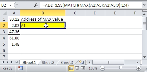
Finding the Address of the Maximum Value in a Range
Suppose you have values in the range A1:A5 and you want to find the address of the cell with the greatest value:
=ADDRESS(MATCH(MAX(A1:A5),A1:A5,0),1,4)

Finding the Address of the Minimum Value in a Range
Similarly, to find the address of the cell with the smallest value in the range A1:A5:
=ADDRESS(MATCH(MIN(A1:A5),A1:A5,0),1,4)

The ADDRESS function is versatile and can be combined with other functions like MATCH and INDEX to dynamically reference cells based on criteria. It is particularly useful in large datasets where cell references need to be generated programmatically.


Leave a Reply