How to Format Your Excel Worksheet?
In this lesson, you will learn everything about formatting in Excel.
Table of Contents
Two Ways to Format in Excel
Formatting in Excel can be accomplished in two ways:
- Using Predefined Styles: This approach is ideal for novice users who rely on standard tables and charts.
- Custom Formatting: If you need full control over your worksheet’s appearance, choose custom formatting. We’ll discuss predefined styles at the end of this lesson.
Method 1: Step-by-Step Formatting
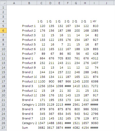
Let’s assume we’ve been tasked with creating a table of data as shown below. We’ve collected the relevant data and inserted them into the table. However, the table has several issues.

Adjusting Column and Row Widths
First, let’s ensure that all data and category descriptions are fully visible. Currently, data in cells ‘I23’ and ‘I32’ are cut off and replaced by ‘###’.
Similarly, descriptions in cells B10 and B32 are also partially obscured. To expand a column, simply double-click on the dash between columns, or click and drag the left button to adjust the width manually.

To make columns equally wide, select the columns you want to align and adjust any of them to the desired size.

Inserting/Deleting Rows
Next, we’ll remove the first three rows at the beginning of the table. To do this, select the first three rows, right-click, and choose Delete.

You can also insert rows or columns using the Insert command. Let’s insert a row above the table.

Adding Borders
When we insert a row at the beginning, Excel selects the entire table. Click on the Borders option, then choose All Edges and Thick Border to make the borders bold.

You can also select the column headers and apply bold borders. No need to reopen the Borders menu; the last selected options can be applied directly.

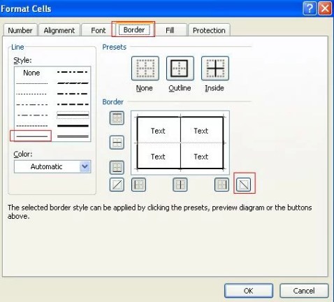
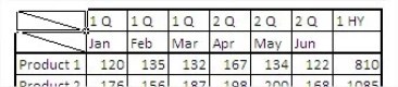
If you require dual or diagonal lines within cells, right-click on a selected cell or area, then choose Format Cells.

In the Format Cells dialog, navigate to the Border tab to explore various border formatting options.
Merging Cells
Merge & Center deserves special mention. This combines multiple cells into one and centers the content.
Select from that cell across to the rightmost cell you want it to span and click Merge & Center.


If you wish to adjust the vertical alignment of merged cells, right-click, choose Format Cells, and set the vertical alignment.

Changing Cell Background Color
To change a cell’s background color, select the cell or area, click the Fill Color option, and choose the desired color.

For subsequent cells, click the Fill Color icon, and it will remember your previous choice.

Using Format Painter
To apply the same format to multiple cells or areas, use the Format Painter. First, format one cell (e.g., line 21) as desired.

Then, click the Format Painter icon and click on the target cell or area to apply the format.

Click in cell B25 and the entire row of the table takes the appropriate format.

Gridlines and Font Size
To improve the document’s appearance, you can disable gridlines and adjust font size easily.


To hide or reveal rows and columns, select them accordingly.


Method 2: Formatting as a Table
For more complex tables, you can format them as tables. Activate a cell within the table, go to Home, select Format as Table, and choose a color scheme. Ensure that the table area is correctly recognized. If needed, you can remove filter symbols from header cells.

A window will appear, in which we are asked to confirm whether the area of the table was properly recognized.

The table is formatted according to the selected model. If it does not suit us, that header cells contain symbols of the filter can be disabled by selecting Sort & Filter and then click Filter.

When you click the right mouse button on the table, we can add a row sum, as is shown below.

Sum which will be introduced only for June, copy to the other months.

Exercise can be considered completed.

On the Design click on the arrow marked below to view all available styles.

Choose the style that suits you.

Select the title by clicking on it and the cards Format select one of the Word Art styles.

Keep in mind that impressing recipients with elaborate styles should not come at the cost of a professional approach. Simplicity often speaks louder than complexity in Excel formatting.


Leave a Reply