How to Use the Average Function in Excel
In this lesson, you can learn how to use the Average function. The average function in Excel is a feature that would use the arguments to return with average of those arguments. However, it would only use the cells that are containing numbers to calculate the average.
The advantage of this function is that it can enter addresses of individual cells and also the whole range. Average is also available in the status bar.
Table of Contents
What is the AVERAGE function in Excel?
The AVERAGE function takes a range of numbers as an argument and returns the average value. The average is calculated by adding all the numbers in the range and then dividing by the number of numbers.
The AVERAGE function works by first adding all the numbers in the range. Then, it divides the sum by the number of numbers.
Syntax of the AVERAGE Function
Parameters (Syntax) The syntax of average has one obligatory argument, while others are optional.
The syntax looks like this: =AVERAGE(number1, [number2], …).
Number1: This is a required argument, and could be cell reference, a range that you would like to have the average of.
Number2: This is optional. It could also contain reference, range, and these ones reach maximum of 255.

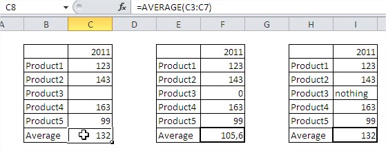
Take a look at the picture above.
Function AVERAGE doesn’t care about empty cells and text in the cell. In the first and third table function AVERAGE there is a different average than in the second table.
It is very easy to make a mistake. Remember about zeros in cells.
Examples of Average function
Average Between Two Values
{=AVERAGE(IF((A1:A10>=B1)*(A1:A10<=B2),A1:A10))}
B1 and B2 are the values between which you want to calculate average.
This is an array formula so accept it by CTRL + SHIFT + ENTER.
To avoid errors
Use this formula when you can haven’t got any data in your worksheet.
=IF(ISERROR(AVERAGE(A1:A5)),”No Data”,AVERAGE(A1:A5))
If your data in A1:A5 are missing, Excel will show “No data”. If it is ok with your data there will be average calculated.
For calculating the average of values within a specific range of criteria, the AVERAGEIFS function is more appropriate.
Average of 10 largest values
{=AVERAGE(LARGE(A1:A50,ROW(1:10)))}
This formula gives you the average of 10 largest values in A1:A50 range as the result.
Average with some data missing
How to calculate values average in case of zeros or missing data. Use that formula:
{=AVERAGE(IF($A$1:$A$5<>0,$A$1:$A$5))}

This formula doesn’t count blanks and zeros. In this case average is (2+5+6+3):4. Formula doesn’t calculate value in A2 cell. There will be the same when A2 will be blank or text.
For multiple criteria, use AVERAGEIFS, which allows specifying one or more ranges and conditions without array formulas:
=AVERAGEIFS(average_range, criteria_range1, criteria1, [criteria_range2, criteria2], …)

Leave a Reply