Why Does VLOOKUP Give Me the Wrong Value?
VLOOKUP is one of the most powerful and easily accessible Excel formulas available. Capable of quickly scanning thousands of rows to almost immediately pull the desired information into a new cell, VLOOKUP should be in every Excel user’s arsenal. If you’re not familiar with the VLOOKUP formula, it can often feel intimidating, especially if you’ve run across your first real need to use it.
Novice VLOOKUP users often get the formula wrong, resulting in pulling either no value or the wrong value. Let’s take a look at some of the most common VLOOKUP mistakes and how to avoid them in the future.
Table of Contents
What is VLOOKUP?
By definition, VLOOKUP formula looks for a value in the leftmost column of a table, and then returns a value in the same row from a column you specify. Simple enough, but let’s break down the actual formula to see where common problems can arise.
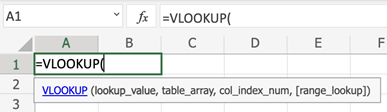
VLOOKUP is broken into four separate parts, and it’s important to have a good grasp of each part.

Here’s the tutorial on how to use vlookup in Excel.
Possible reasons
First, you need to identify the lookup value. This is the value that you want the formula to scan and identify in a range of data. When it identifies the lookup value, it will then pull a piece of information in the same row as that lookup value, which you specify later in the formula.
As an example, the below formula is pointing to D2, meaning the formula needs to first look for Ted in the range we specify.

A common error that users make is not understanding the lookup_value command of the formula. It may seem like it’s asking what information to find and pull into the cell (after all, it’s asking what to look up in the range). A novice user may instinctually put a cell other than D2 in the lookup_value part of the formula, such as B2 to look up the ID, producing an error.
Second in the formula is the range in which you want to search for the output. In this example, we are looking at columns A through B. For longer sets of data, the lookup_value may not always be in the first column of the range. It’s important to always use the column where the lookup_value is found as the first column in the range.
For example, if column A was the Department an employee works in, Column B is their name, and Column C is their ID, we would enter range B:C since we are looking up the output by the Name (cell D2). A common issue is highlighting the enter range of data, resulting in an error.
Third in the formula is the column that houses the information (the col_index_num) you want to extract into the cell. In this example, we want the ID to be the output. The ID column is the second column in the range that we identified, meaning we would put a 2 for the col_index_num. It’s common to see an incorrect number entered here, especially for larger sets of data with many columns.
The last piece of the formula is the range_lookup, which is determined by entering TRUE or FALSE. By entering FALSE, you’re specifying that the lookup_value must be an exact match in the range of data you’re reviewing. If you enter TRUE, Excel will find the closest match, which may not be exact. This distinction is crucial for ensuring the accuracy of the returned value.
To correct the issue with the VLOOKUP function giving you the wrong value, you need to go through each of these potential issues and make the necessary changes to your VLOOKUP function. This may require checking the data types, sorting the table array, adjusting the range_lookup argument, and more.


Leave a Reply