How to Define a Custom Number Format in Excel
In Excel, you can define custom number formats to display numbers in a specific way. This can be useful for formatting currency, percentages, dates, and times.
You will learn how to define a custom number format in Excel. You will also learn about the most commonly used codes for custom number formats.
Number format creation
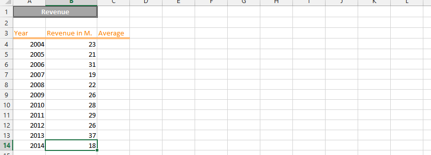
To define a custom number format prepare the data.

Select the cells that you want to format.

Click the Format Cells button.

In the Number tab, select the Custom category. In the Type field, enter the custom format code.
Most commonly used codes
Some of the most commonly used codes include:
- #: Represents a digit placeholder.
- 0: Represents a digit placeholder, but if a number has fewer digits than there are digit placeholders, the extra placeholders will be filled with zeros.
- . (period): Specifies the position of the decimal point in the number format.
- , (comma): Specifies the position of the thousands separator in the number format.
- %: Specifies that the number should be displayed as a percentage.
- $: Specifies that the number should be displayed as a currency value, with the appropriate currency symbol.
When defining a custom number format, you can combine these codes to create a format that meets your specific needs.
Custom format examples
Here are some examples of custom number formats:
- “#,##0.00”: This format displays a number with a comma as the thousands separator and two decimal places.
- “0.0%”: This format displays a percentage with one decimal place.
- “# ???/???”: This format displays a date as a day, month, and year, with a space between each.
Note: You can even format colors. Just write [color]
How to Format Date and Time?
How to Easily Format Date and Time in Excel Format of date and time can be tough, but it will easily be performed together with me, follow me as I format date and time.
Date formatting
Click on a cell, type in =DATE(2014(year);10(month);05(day)).

Time formatting
Click on another empty cell, and type in =TIME(hour;minutes;seconds), and finally press enter.

Right-click on the time, and choose format cells.

Click on date, and choose desired format.

Repeat previous step, but this time choose time, the type you want.

Experiment with the different formatting codes to see how they can work for you.
It’s important to understand that custom number formats only change the display of a value, not the underlying stored value. Calculations will still be performed using the actual numerical value, regardless of the formatting applied.


Leave a Reply