If Function with multiple conditions
In this article, I will guide you to write simple if functions as well as the complex if functions with multiple conditions or we also call it nested if functions.
Lets start with simple if function in Excel formulas:
Basics of if formula with multiple conditions
The syntax is like : =IF( condition, value_if_true, value_if_false)
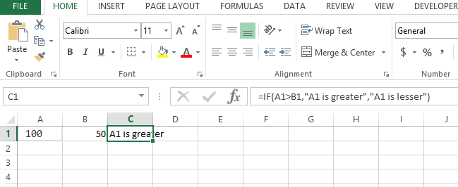
So there are 3 arguments, first is the condition like a>b , second is the result if the condition result is true, 3rd argument is the result if the condition is false. e.g:
=IF(A1>B1,”A1 is greater”,”A1 is lesser”)

Simple example of if formula with multiple conditions
This explains the simple if with one condition but we have more conditions like we also have to check say the difference between the 2 numbers is > 30 of not then we will have to use nested if like:
=IF(A1>B1,IF(A1-B1>30,”difference is >30″,”difference is<30″),”A1 is lesser”)
So we have actually changed the result if true to another if statement like:
=IF(A1-B1>30,”difference is >30″,”difference is<30″)

So the result of first condition A1>B1 if it comes true then it will check the next condition
A1-B1>30 and similarly there are 2 results if this condition is true or false.
VBA code of if formula with multiple conditions
If we have to write this entire thing in vba code or any coding algorithm it will look like this:
If A1> B1 Then

If (A1-B1 ) > 30 Then

Msgbox "difference is >30"

Else

Msgbox "difference is <30"

End if

Else

Msgbox “A1 is lesser”

End if
Based on the code you can see how IF function is nested and how the conditions are being checked.
An alternative solution using the CHOOSE function
Here’s another example of using the IF function with multiple conditions:
Suppose you have a list of student grades in column A, and you want to assign a letter grade to each student based on their numeric score. You can use the following formula in column B to assign letter grades:
=IF(A2>=90,”A”,IF(A2>=80,”B”,IF(A2>=70,”C”,IF(A2>=60,”D”,”F”))))
This formula checks whether the grade in cell A2 is greater than or equal to 90. If it is, the formula assigns an “A” to the student. If the grade is less than 90, the formula checks whether it’s greater than or equal to 80. If it is, the formula assigns a “B” to the student. The same logic follows for grades of 70 or higher, 60 or higher, and below 60. If the grade is below 60, the formula assigns an “F” to the student.
It looks to compilated to me.
Here’s an alternative solution to assign letter grades to student grades using the CHOOSE function in Excel:
=CHOOSE(INT((A2-50)/10)+1,”F”,”D”,”C”,”B”,”A”,”A”)
This formula takes the student grade in cell A2 and divides it by 10, subtracts 5, and rounds down to the nearest integer. The resulting number is used as an index to the CHOOSE function, which returns the corresponding letter grade based on the following logic:
- If the rounded-down grade is less than 0 or greater than 5, the formula returns “F”.
- If the rounded-down grade is 0, the formula returns “D”.
- If the rounded-down grade is 1, the formula returns “C”.
- If the rounded-down grade is 2, the formula returns “B”.
- If the rounded-down grade is 3 or greater, the formula returns “A”.
You can drag this formula down to the rest of the cells in column B to apply it to the entire list of student grades.
This alternative looks easier to me.


Leave a Reply