How to Refresh Data in Pivot Table
In this Excel tutorial, you learn how to refresh pivot table with new data. You need this to analyze the data after the update.
Table of Contents
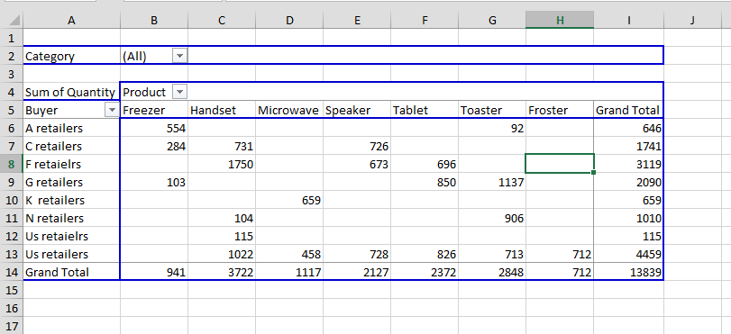
Pivot Table data preparation
Click any cell in the pivot table.

After clicking the cell, Pivotable Tools will appear in the toolbar. Click Analyze under PivoTtable Tools.

Refreshing pivot table data
Click refresh to refresh your data in the pivot tables. This will refresh the data in the pivot table with the latest data in the source range.
Note: For large pivot tables, it may take a long time.
To have refreshed data by default, go to PivotTable Options and tick the “Refresh data when opening the file” option.

You may think about unticking this option when you are opening the huge datasets many times a day. Refreshing may be a major part of your workday.


Leave a Reply