How to Vlookup Backwards
Something tricky today. Let’s create some backwards VLOOKUP formula. It’s quite easy, but not obvious. Here’s an example.
Vlookup is a powerful function in Excel that can be used to search for a specific value in a range of cells and return a corresponding value from a different column in the same row.
By default, Vlookup searches for values in the first column of a range and returns the corresponding value from a specified column. However, sometimes you may want to search for a value in a column to the right of the range and return a corresponding value from a column to the left.
Table of Contents
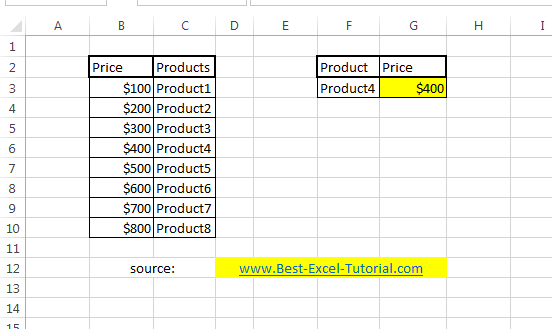
Sample dataset for Vlookup
The sample data table shows the products and prices. You try to find the price.

Backwards Vlookup formula
To perform a “Vlookup backwards” in Excel, you can use the INDEX and MATCH functions together. The INDEX function can return a value from a specific cell within a range of cells, while the MATCH function can search for a value within a range of cells and return its relative position.
By combining these two functions, you can create a Vlookup-like function that works in reverse.
The formula of reverse VLOOKUP is: =INDEX($C$3:$C$10,MATCH($F$3,$B$3:$B$10,0))
Explanation:
- C column – prices – array where you have your values whose you are looking for.
- B column – products – names of all products which prices you know.
- F3 – name of the product, which price you are looking for.
Now you know how to do a reverse VLOOKUP in Excel using INDEX and MATCH functions.
This is a simple example of how to perform a Vlookup backwards in Excel. You can modify the formula and the data as needed for your specific requirements.
Note: The above formula will return an error if the value being searched for does not exist in the search range. To avoid this, you can wrap the formula in an IFERROR function.


Leave a Reply