How to do a Vlookup with Multiple Criteria
In this Excel tutorial, you will learn how to do a vlookup with multiple criteria in Excel.
Using CONCATENATE for Multiple Criteria VLOOKUP
Data Preparation
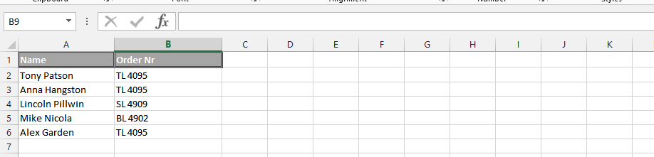
Begin with a dataset containing multiple columns, including the criteria you want to match.

Inserting a Concatenate Formula
Insert a new column by right-clicking on an existing one.

In the newly inserted column, create a concatenate formula using the CONCATENATE function (e.g., =CONCATENATE(B6, C6)) to combine the values of the criteria columns for each row.

Inserting Vlookup formula
In separate cells, enter the specific criteria you want to search for (e.g., “Tony” and “Olson”).

In an empty cell, use the VLOOKUP function to search for the concatenated criteria in your dataset. The formula should look like this: =VLOOKUP(B3&C3, $A$5:$E$10, 5, FALSE).

Replace “B3&C3” with the cell references containing your criteria.
Adjust the range and column number as needed based on your dataset.
While using a helper column is often the simplest approach, you can also achieve a many-to-many lookup without a helper column using INDEX/MATCH and array formulas. This method is more complex but can be useful when modifying the original data structure is not an option.


Leave a Reply