How to Use VLOOKUP in Excel
VLOOKUP is a powerful Excel function that allows you to search for a specific value in the first column of a table array and retrieve a corresponding value from a different column within the same table array. This guide will provide an in-depth understanding of VLOOKUP, its parameters and how it works.
What is the VLOOKUP function in Excel?
VLOOKUP stands for Vertical Lookup. It is a function that takes three arguments:
- The value you are looking for
- The range of cells that contains the values you are looking for
- The column number of the value you want to return
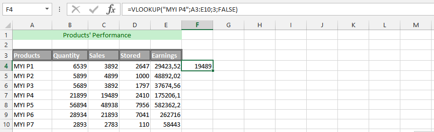
For example, if you have a table of products and their prices, and you want to find the price of the product with the SKU “12345”, you would use the following formula:
=VLOOKUP(“12345”, “Products”, 2)
This formula would return the value in the second column of the Products range that matches the value “12345” in the first column.
Understanding the VLOOKUP function and its parameters
The VLOOKUP has multiple parameters that work together to find the value that the user is looking for with it. The function has a lookup value, a table of array, index’s column number, and a range lookup.
Lookup Value: This is a value that a user searches for in the first column of a table’s array. This can be either a reference or a value. If there was a lookup value that was smaller than the smallest value in the same first column of that table array, it would only lead to the VLOOKUP returning with the #N/A error value.
Table Array: There needs to be either two or more columns that contain data. It is possible for this to be either a range name or a range reference. Values that are in this array’s first column would be searched by a lookup array. These values can be logical values, numbers, or even text.
The array is equal to both the upper- and lowercase text.
Column Index Number: This is a column number that is in the table array, which is where a matching value is required to be matched.
If it is 1, then it would return a value that is in the first column of that table’s array. If it is 2, then it would return with the second column in the array; if it is 3, it will return with the third column, and so on. When it is less than 1, then it will be returned with an error value that says #Value!
However, if the number is greater than the number of columns in a table’s array, then the VLOOKUP function would return with the error value that says #REF!
Range Lookup: This is the logical value that would be specified if the user wants the VLOOKUP function to either find the exact match of the value or just make an approximating match.
How the VLOOKUP function works in Excel
VLOOKUP works by first searching for the value you are looking for in the first column of the range you specify. If it finds a match, it returns the value in the column you specify. If it doesn’t find a match, it returns an error value.
Exact match in Excel VLOOKUP
By default, VLOOKUP performs an exact match. This means that the value you are looking for must match the value in the first column of the range exactly. If there is any difference, VLOOKUP will not return a match.
You can force VLOOKUP to perform an approximate match by setting the fourth argument to TRUE. This will allow VLOOKUP to return a match even if the value you are looking for is not an exact match.
Excel alternatives to VLOOKUP
There are a few alternative functions to VLOOKUP. These include:
- HLOOKUP: This function works the same way as VLOOKUP, but it looks up a value horizontally across a table.
- INDEX MATCH: This function is more flexible than VLOOKUP, but it is also more complex to use.
- MATCH: This function can be used to find the position of a value in a range, without returning the value itself.


How To VLOOKUP In Pandas • Pandas How To
[…] The `merge` method in Pandas is the equivalent of the VLOOKUP function in Excel. […]