How to Insert Checkbox in Excel
A check box is a form control that allows users to select or deselect an option. Check boxes can be used to create interactive forms, surveys, and data filters. In this lesson, you will learn how to insert check box to the worksheet in Excel.
Why use check boxes?
Check box enables or disables a value indicating alternatives with a specific meaning. In the worksheet or in a group box you can tick more than one box at a time. The check box can be used, for example in the order form containing a list of available products or inventory tracking application to indicate whether a particular product has been discontinued.
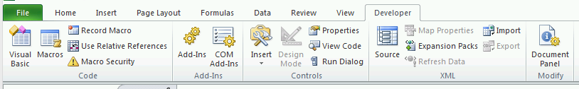
Go to the Ribbon > Developer tab.

How to insert a check box
Click Insert and select a form control check box and place it on the sheet.

By right-clicking on a control you can edit the name of the button, the assigned macro, and other parameters. Click the Format Control.

You will see a window object formatting. Go to the tab control fill in the cell link pointing to a cell in the spreadsheet link eg C2. You can specify the cell link that will be updated with the checkbox status (either True or False). Additionally, you can set other options such as the checkbox size, font, and font color.

You connected a link to cell C2, which according to click on a checkbox appears logical value “TRUE” or “FALSE”.
False

True

You can create interactive and functional checkboxes in your Excel worksheets.


Leave a Reply