How to use Conditional Formatting in Excel
In this lesson, you will learn how to use conditional formatting. Harness conditional formatting to highlight critical values, reveal trends, and compare data automatically.
Table of Contents
Conditional Formatting in Excel
Excel is a powerful tool for capturing, analyzing, and visualizing data. With countless tools at your disposal, you can leverage Excel to tell accurate stories with the data you have available. Conditional formatting is a popular Excel tool that takes visualization one step further.
Rather than diving into the details of the data, conditional formatting allows you to efficiently understand data in relation to the rules and parameters you set. For example, you can set conditional formatting to visually identify values that either increase or decrease when compared to something else in the sheet. Let’s take a look at how that happens.
Conditional formatting automatically applies formatting to cells based on specified criteria. For example, you can change the background color of all cells with values greater than 100. This feature is a powerful tool for data analysis and visualization.
Conditional formatting is a powerful Excel tool that allows you to automatically format cells based on certain conditions. This can be used to highlight important data, identify trends and make your spreadsheets more visually appealing.
To use conditional formatting, first select the cells you want to format. Then, click on the Home tab and select Conditional Formatting. You can choose from a variety of formatting options, such as changing the font color, background color or cell borders. You can also use conditional formatting to create icons or sparklines.
Here are some examples of how you can use conditional formatting:
- Highlight cells that contain values above or below a certain threshold.
- Identify duplicate values.
- Show trends over time.
- Flag important data.
Conditional formatting is a versatile tool that can be used to improve the readability and usability of your spreadsheets. With a little practice, you can learn to use it to create effective and visually appealing visualizations of your data.
Basic conditional formatting in Excel
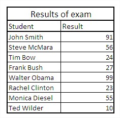
I prepared a table with the results of the exam.

You want to highlight the extreme results. The best results are highlighted in green if they are above 90% and in red if they are below 30%. How to do it?
The conditional formatting button is at the center of the Excel ribbon.

Start with the best students. All results with a score of 90% or higher want to paint the color green. Click on the button Conditional Formatting on the ribbon and select Greater Than.

A dialog box appears. The entry requirement is 90%. Select the format of a custom list to determine the green fill.

Similarly, do so with the next conditions. Less than 30% of those polled chose to fill in the red.

Excel automatically applies the formatting you specify to the cells that meet the condition.
Advanced conditional formatting in Excel
Other (example) formatting options are presented in the following figure.

I used blue stripes to format the first column. The length of the stripes increases as the value in the cell increases. This option can be turned on in a way that I showed in the picture.

The second column’s formatting benefited from the color scale. On only the first scale, the highest values are green and the lowest are red.

The results in the third column are formatted using icon sets. Icon sets can be a fun way to visualize data, but they may not be appropriate for all workplaces.
![]()
Show an Increase or Decrease in Conditional Formatting
In this example, we’ll take a look at sales numbers and how to use conditional formatting to identify increases or decreases compared to average sales volumes.
Before you set the conditional formatting rules, make sure your data is formatted correctly. We are going to compare monthly sales volumes against average sales volumes, as seen below.

We will use conditional formatting to easily identify the numbers in the Sales by Month column. The example shows the Average Sales Volume number that will allow us to set a conditional formatting to compare an increase or decrease.
In Excel’s Home tab, select Conditional Formatting, then select New Rule. Select the range of cells you want to format (in this case, the cells in the Sales by Month column). For Rule Type, select Highlight Cells With, then select Cell Value Greater Than. Finally, select the Average Sales Volume as the target cell.

This rule will highlight any increases in the sales volume. To identify decreases compared to the average, simply create a second rule. Rather than selecting Greater Than, simply select Less Than. These two rules will quickly highlight increases and decreases, so you don’t need to assess every line item.

Conditional Formatting for a row
You are going to learn, how to format whole row not only one cell. It can be useful for some reports or presentations.

You have an Excel sales report.

You can format rows with sales greater than $10,000 in Excel. First select your data without headings.

Next go to the ribbon and click Conditional Formatting and New Rule.

On the dialog box choose Use a formula to determine which cells to format option.

Write down =$B5>$C$2 formula.

Next, click Format and choose how your rows will be formatted. I clicked Fill and chose yellow background.

Click OK to see your Excel data formatted.

Practical Applications in Business: Next Steps
Now that you understand the fundamental concepts of this Excel feature, the next logical step is to apply them to real-world business scenarios and advanced analysis. Our comprehensive learning hubs show how professionals use these foundations to build dashboards, analyze data, and make strategic decisions.
📊 Explore Business Applications:
- Excel for Business Intelligence & KPI Dashboards – Learn how companies use these fundamentals to build real-time performance dashboards, track metrics, and drive data-driven decisions. Perfect for managers, analysts, and business users building professional dashboards.
- Excel for Personal Finance & Investing – Apply Excel skills to financial planning, investment analysis, and portfolio tracking. Essential for anyone managing personal wealth or analyzing financial data.
- Excel for Data Analysis & Statistics – Combine these concepts with statistical methods for advanced analysis, forecasting, and data interpretation. Required for data analysts and researchers.
These hubs bridge the gap between Excel basics and professional applications. Start with the hub that matches your role or goals—each provides step-by-step guidance and real-world examples.


Leave a Reply