How to calculate XIRR Annualized Return
The understanding of the usefulness of the XIRR function in Excel varies for different reasons. There are some that would find it useful for one thing, while it might be useful for other things. It is practically useful for anything that has to do with calculating your returns.
When it comes to investing money, there are actually differences in time value. When depositing and withdrawing money and then receiving dividends, it becomes much more difficult to make the calculation of the annualized returns.
This is because there is certainly a difference between making an investment of $1,000 in January and investing the same amount in December, right before the year ends. This makes the XIRR feature of Microsoft Excel something that simplifies the calculation.
How to calculate XIRR for Annualized Returns?
When all the data has been gathered, it would be easy to calculate the annualized return. This is because the true returns of any portfolio will include all cash flows, and the XIRR function in Excel is best suited for calculating the returns.
If it happens, the return calculation would be as simple as taking the beginning balance and ending balance, and then finally calculating the absolute return, which would make tracking investment returns so much easier.
Now we will perform the XIRR calculation in Excel to determine annualized investment returns based on cash flow timing and investment amounts.
Necessary Data
This is the first step to using the XIRR feature in Microsoft Excel. The data has to be directly relevant for the calculation to be made. The relevance is flexible and dependent on the timing of each investment. I want to know my XIRR annualized returns for the last year, which makes it possible for the calculation to be quite different.
It is possible for your calculation to produce a whole new result, because it has to do with the date. This is because it is natural for you to set the date between January 1st and December 31st.

Understanding investment dates is critical for XIRR calculations because the date of each cash flow significantly affects annualized returns—investments made at the year’s beginning versus year-end produce different return percentages and require precise date-weighted analysis.
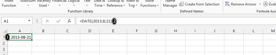
You should click on the column as it is marked with the number 1, and then type in =date (year; month; date) in that same column, as it is showing in the area labeled as number 2. You should follow these steps to calculate all the dates on which the investments were made.

Click on the column that is beside a specific date, as it is labeled as number 1, and then surrounded in green. You should type in the amount, as it is shown in number 2. It is important to know the amount invested on that very same day.
As you can see, we have placed a subtraction in front of the column. This is to make it possible for you to familiarize yourself with a scenario where there is subtraction prior to the investments.
Calculation of the Annualized XIRR
This is where we would now calculate your annual returns with the XIRR feature.
The syntax for the XIRR function is as follows:
=XIRR(values, dates, [guess])
Where:
- Values: The range of cells containing the cash flows.
- Dates: The range of cells containing the dates of the cash flows.
- Guess: An optional argument representing your estimate of the annualized return. If omitted, Excel will use 0.1 (10%) as the default guess.

Click on any empty column, as was the case, in the place labeled as number 1, and then type in =XIRR (value; dates) in that column, as it is displayed in the area labeled as 2, and then press enter. It is important to first choose all the values and then place them in the same row.

Click on the column beside the calculation you made in the previous step, as it is in the area marked as number 1, and type in XIRR. This allows you to know which column has the calculation in it. Right-click with the mouse on the column you’d calculated, as labeled as number 2, and then choose Format Cells, which is number 3.

In the Format Cells dialog, navigate to the Number tab and select Percentage format with two decimal places to display the XIRR calculation result as an annualized percentage return, then click OK to apply this Excel formatting.
You have now successfully completed the XIRR calculation process, which provides an accurate measurement of annualized returns on your investment portfolio by accounting for both the timing and amount of each cash flow.

Leave a Reply