How to VLOOKUP Zip Codes?
Whether for a school project or a work assignment, chances are you’re going to need to use VLOOKUP at least once in your life. Let’s say you have a long list of names, contact information, and addresses, including zip codes.
You need to pull the zip codes for a targeted subset of contacts on the list, but looking up each contact individually is time consuming. Fortunately, VLOOKUP can help you quickly pull zip codes for any sized list of contacts. Let’s take a look how to VLOOKUP zip codes.
Start by organizing your data into two separate Excel lists. The first list should contain a list of zip codes, and the second one should contain the information you want to return based on the zip code, such as the city, state, or latitude and longitude coordinates.
Table of Contents
Zip codes task
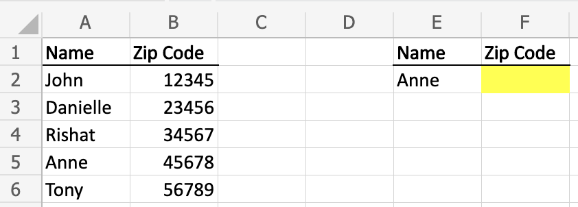
In this example, you have a list of contacts and need to quickly identify Anne’s zip code from the contact sheet. For this example, we are using a short list for simplicity, but the same concepts can be used if the list is 10 rows long or 10,000 rows long.
Learning materials are available under this link.

First, we need to identify what we are looking for. In this example, we are using VLOOKUP to identify Anne’s zip code.
In order to identify her zip code, we need to understand the VLOOKUP formula.
A VLOOKUP formula looks for a value in the leftmost column of a table, and then returns a value in the same row from a column you specify. It is broken up into four distinct parts (the value, the range you’re looking in, the column that houses the information you want to pull into the cell, and whether or not you need an exact match of what the value is).

Vlookup zip code formula
To successfully pull in Anne’s zip code, structure the formula as follows: =VLOOKUP(E2,A:B,2,FALSE)
- E2 – points to Anne, meaning we are looking up Anne in our range
- A:B – the range of columns to search. Column A contains the names, and column B contains the zip codes.
- 2 – specifies that the zip code is in the second column of the range.
- FALSE – Ensures an exact match. If Anne’s name is not found or spelled differently, no value will be returned.

To make it easier to identify the information returned based on the zip code, you can use conditional formatting. Conditional formatting allows you to apply a fill color, font color, or other formatting to a cell or range of cells based on a condition.
Conditional formatting can help you quickly identify the cells containing zip codes or any other specific information.


Leave a Reply