How to Freeze Panes and Split in Excel
Freezing panes and splitting the worksheet in Excel are useful features that help you navigate and work with large datasets more effectively.
Here’s how to freeze panes and split the worksheet.

You have quite a large table that does not fit in the Excel. For this reason, you do not see headers and it is hard you work. The table in this form is completely unreadable.
Freeze Panes
Freezing panes allows you to keep specific rows or columns visible while scrolling through a large Excel worksheet. This is especially helpful when you want to keep headers or labels visible as you scroll.

You can choose one of the following options:
- “Freeze Panes” will freeze both the rows above and the columns to the left of your selection.
- “Freeze Top Row” will freeze only the rows above your selection.
- “Freeze First Column” will freeze only the columns to the left of your selection.
Choose Freeze Panes.

Excel will freeze the selected rows and columns, making them visible as you scroll through your worksheet.

Worksheet Split
Splitting the worksheet allows you to view different sections of the same worksheet simultaneously. This is helpful when you want to compare data from different parts of the worksheet or work with large datasets more efficiently.
In the “Window” group, click on “Split”.

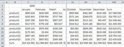
The worksheet will be split into separate panes, allowing you to view different parts of the worksheet at the same time.
After applying the Split, your worksheet will be divided into four independently scrollable sections. This functionality is particularly beneficial when analyzing large datasets, as it allows for simultaneous comparison of data from different worksheet areas.

You can adjust the split by clicking and dragging the split bars that appear on the worksheet. This allows you to control the size and position of each section.
You can use both freeze panes and split worksheet features in Excel to work more efficiently and make it easier to view and analyze your data.


Leave a Reply